Normal Distribution Probability Plotting Example

New format available! This reference is now available in a new format that offers faster page load, improved display for calculations and images and more targeted search.

As of January 2024, this Reliawiki page will not continue to be updated. Please update all links and bookmarks to the latest references at Weibull examples and Weibull reference examples.

---

This example appears in the Life data analysis reference.

7 units are put on a life test and run until failure. The failure times are 85, 90, 95, 100, 105, 110, and 115 hours. Assuming a normal distribution, estimate the parameters using probability plotting.

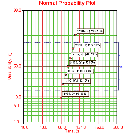
In order to plot the points for the probability plot, the appropriate estimates for the unreliability values must be obtained. These values will be estimated through the use of median ranks, which can be obtained from statistical tables or from the Quick Statistical Reference (QSR) tool in Weibull++. The following table shows the times-to-failure and the appropriate median rank values for this example:

[math]\displaystyle{ \begin{matrix} \text{Time-to-} & \text{Median} \\ \text{Failure (hr)} & \text{Rank ( }\!\!%\!\!\text{ )} \\ \text{85} & \text{ 9}\text{.43 }\!\!%\!\!\text{ } \\ \text{90} & \text{22}\text{.85 }\!\!%\!\!\text{ } \\ \text{95} & \text{36}\text{.41 }\!\!%\!\!\text{ } \\ \text{100} & \text{50}\text{.00 }\!\!%\!\!\text{ } \\ \text{105} & \text{63}\text{.59 }\!\!%\!\!\text{ } \\ \text{110} & \text{77}\text{.15 }\!\!%\!\!\text{ } \\ \text{115} & \text{90}\text{.57 }\!\!%\!\!\text{ } \\ \end{matrix}\,\! }[/math]

These points can now be plotted on a normal probability plotting paper as shown in the next figure.

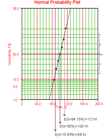
Draw the best possible line through the plot points. The time values where the line intersects the 15.85%, 50%, and 84.15% unreliability values should be projected down to the abscissa, as shown in the following plot.

The estimate of [math]\displaystyle{ \mu \,\! }[/math] is determined from the time value at the 50% unreliability level, which in this case is 100 hours. The value of the estimator of [math]\displaystyle{ \sigma \,\! }[/math] is determined as follows:

[math]\displaystyle{ \begin{align} \widehat{\sigma }= & \frac{t(Q=84.15%)-t(Q=15.85%)}{2} \\ \widehat{\sigma }= & \frac{112-88}{2}=\frac{24}{2} \\ \widehat{\sigma }= & 12\text{ hours} \end{align}\,\! }[/math]

Alternately, [math]\displaystyle{ \widehat{\sigma }\,\! }[/math] could be determined by measuring the distance from [math]\displaystyle{ t(Q=15.85%)\,\! }[/math] to [math]\displaystyle{ t(Q=50%)\,\! }[/math], or [math]\displaystyle{ t(Q=50%)\,\! }[/math] to [math]\displaystyle{ t(Q=84.15%)\,\! }[/math], as either of these two distances is equal to the value of one standard deviation.