Simple Linear Regression Analysis: Difference between revisions
Lisa Hacker (talk | contribs) No edit summary |
|||
| (389 intermediate revisions by 8 users not shown) | |||
| Line 1: | Line 1: | ||
= | {{Template:Doebook|3}} | ||
Regression analysis is a statistical technique that attempts to explore and model the relationship between two or more variables. For example, an analyst may want to know if there is a relationship between road accidents and the age of the driver. Regression analysis forms an important part of the statistical analysis of the data obtained from designed experiments and is discussed briefly in this chapter. Every experiment analyzed in a [https://koi-3QN72QORVC.marketingautomation.services/net/m?md=Rw01CJDOxn%2FabhkPlZsy6DwBQ%2BaCXsGR Weibull++] DOE foilo includes regression results for each of the responses. These results, along with the results from the analysis of variance (explained in the [[One Factor Designs]] and [[General Full Factorial Designs]] chapters), provide information that is useful to identify significant factors in an experiment and explore the nature of the relationship between these factors and the response. Regression analysis forms the basis for all [https://koi-3QN72QORVC.marketingautomation.services/net/m?md=Rw01CJDOxn%2FabhkPlZsy6DwBQ%2BaCXsGR Weibull++] DOE folio calculations related to the sum of squares used in the analysis of variance. The reason for this is explained in [[Use_of_Regression_to_Calculate_Sum_of_Squares|Appendix B]]. Additionally, DOE folios also include a regression tool to see if two or more variables are related, and to explore the nature of the relationship between them. | |||
This chapter discusses simple linear regression analysis while a [[Multiple_Linear_Regression_Analysis|subsequent chapter]] focuses on multiple linear regression analysis. | |||
Regression | ==Simple Linear Regression Analysis== | ||
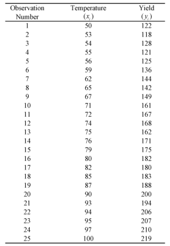
A linear regression model attempts to explain the relationship between two or more variables using a straight line. Consider the data obtained from a chemical process where the yield of the process is thought to be related to the reaction temperature (see the table below). | |||
[[Image:doet4.1.png|center|343px|Yield data observations of a chemical process at different values of reaction temperature.|link=]] | |||
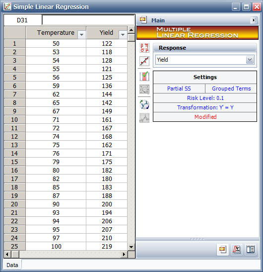
This data can be entered in the DOE folio as shown in the following figure: | |||
[[Image:doe4_1.png|center|530px|Data entry in the DOE folio for the observations.|link=]] | |||
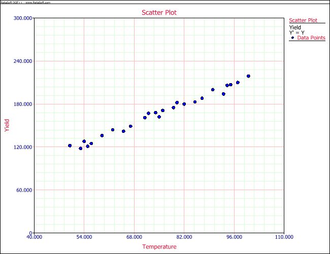
And a scatter plot can be obtained as shown in the following figure. In the scatter plot yield, <math>y_i\,\!</math> is plotted for different temperature values, <math>x_i\,\!</math>. | |||
[[Image:doe4_2.png|center|650px|Scatter plot for the data.|link=]] | |||
It is clear that no line can be found to pass through all points of the plot. Thus no functional relation exists between the two variables <math>x\,\!</math> and <math>Y\,\!</math>. However, the scatter plot does give an indication that a straight line may exist such that all the points on the plot are scattered randomly around this line. A statistical relation is said to exist in this case. The statistical relation between <math>x\,\!</math> and <math>Y\,\!</math> may be expressed as follows: | |||
::<math>Y=\beta_0+\beta_1{x}+\epsilon\,\!</math> | |||
The above equation is the linear regression model that can be used to explain the relation between <math>x\,\!</math> and <math>Y\,\!</math> that is seen on the scatter plot above. In this model, the mean value of <math>Y\,\!</math> (abbreviated as <math>E(Y)\,\!</math>) is assumed to follow the linear relation: | |||
::<math>E(Y) = \beta_0+\beta_1{x}\,\!</math> | |||
The actual values of <math>Y\,\!</math> (which are observed as yield from the chemical process from time to time and are random in nature) are assumed to be the sum of the mean value, <math>E(Y)\,\!</math>, and a random error term, <math>\epsilon\,\!</math>: | |||
The actual values of <math>Y </math> | |||
::<math>\begin{align}Y = & E(Y)+\epsilon \\ | |||
= & \beta_0+\beta_1{x}+\epsilon\end{align}\,\!</math> | |||
The | The regression model here is called a ''simple'' linear regression model because there is just one independent variable, <math>x\,\!</math>, in the model. In regression models, the independent variables are also referred to as regressors or predictor variables. The dependent variable, <math>Y\,\!</math> , is also referred to as the response. The slope, <math>\beta_1\,\!</math>, and the intercept, <math>\beta_0\,\!</math> , of the line <math>E(Y)=\beta_0+\beta_1{x}\,\!</math> are called ''regression coefficients''. The slope, <math>\beta_1\,\!</math>, can be interpreted as the change in the mean value of <math>Y\,\!</math> for a unit change in <math>x\,\!</math>. | ||
The random error term, <math>\epsilon\,\!</math>, is assumed to follow the normal distribution with a mean of 0 and variance of <math>\sigma^2\,\!</math>. Since <math>Y\,\!</math> is the sum of this random term and the mean value, <math>E(Y)\,\!</math>, which is a constant, the variance of <math>Y\,\!</math> at any given value of <math>x\,\!</math> is also <math>\sigma^2\,\!</math>. Therefore, at any given value of <math>x\,\!</math>, say <math>x_i\,\!</math>, the dependent variable <math>Y\,\!</math> follows a normal distribution with a mean of <math>\beta_0+\beta_1{x_i}\,\!</math> and a standard deviation of <math>\sigma\,\!</math>. This is illustrated in the following figure. | |||
[[Image:doe4.3.png|center|583px|The normal distribution of <math>Y\,\!</math> for two values of <math>x\,\!</math>. Also shown is the true regression line and the values of the random error term, <math>\epsilon\,\!</math>, corresponding to the two <math>x\,\!</math> values. The true regression line and <math>\epsilon\,\!</math> are usually not known.|link=]] | |||
===Fitted Regression Line=== | ===Fitted Regression Line=== | ||
The true regression line is usually not known. However, the regression line can be estimated by estimating the coefficients <math>\beta_1\,\!</math> and <math>\beta_0\,\!</math> for an observed data set. The estimates, <math>\hat{\beta}_1\,\!</math> and <math>\hat{\beta}_0\,\!</math>, are calculated using least squares. (For details on least square estimates, refer to [[Appendix:_Life_Data_Analysis_References|Hahn & Shapiro (1967)]].) The estimated regression line, obtained using the values of <math>\hat{\beta}_1\,\!</math> and <math>\hat{\beta}_0\,\!</math>, is called the ''fitted line''. The least square estimates, <math>\hat{\beta}_1\,\!</math> and <math>\hat{\beta}_0\,\!</math>, are obtained using the following equations: | |||
::<math>\hat{\beta}_1 = \frac{\sum_{i=1}^n y_i x_i- \frac{(\sum_{i=1}^n y_i) (\sum_{i=1}^n x_i)}{n}}{\sum_{i=1}^n (x_i-\bar{x})^2}\,\!</math> | |||
::<math>\hat{\beta}_0=\bar{y}-\hat{\beta}_1 \bar{x}\,\!</math> | |||
where <math>\bar{y}\,\!</math> is the mean of all the observed values and <math>\bar{x}\,\!</math> is the mean of all values of the predictor variable at which the observations were taken. <math>\bar{y}\,\!</math> is calculated using <math>\bar{y}=(1/n)\sum)_{i=1}^n y_i\,\!</math> and <math>\bar{x}\,\!</math> is calculated using <math>\bar{x}=(1/n)\sum)_{i=1}^n x_i\,\!</math>. | |||
Once <math>\hat{\beta}_1\,\!</math> and <math>\hat{\beta}_0\,\!</math> are known, the fitted regression line can be written as: | |||
::<math>\ | ::<math>\hat{y}=\hat{\beta}_0+\hat{\beta}_1 x\,\!</math> | ||
where <math>\hat{y}\,\!</math> is the fitted or estimated value based on the fitted regression model. It is an estimate of the mean value, <math>E(Y)\,\!</math>. The fitted value,<math>\hat{y}_i\,\!</math>, for a given value of the predictor variable, <math>x_i\,\!</math>, may be different from the corresponding observed value, <math>y_i\,\!</math>. The difference between the two values is called the ''residual'', <math>e_i\,\!</math>: | |||
::<math>e_i=y_i-\hat{y}_i\,\!</math> | |||
====Calculation of the Fitted Line Using Least Square Estimates==== | ====Calculation of the Fitted Line Using Least Square Estimates==== | ||
The least square estimates of the regression coefficients can be obtained for the data in the preceding [[Simple_Linear_Regression_Analysis#Simple_Linear_Regression_Analysis| table]] as follows: | |||
::<math>\begin{align}\hat{\beta}_1 = & \frac{\sum_{i=1}^n y_i x_i- \frac{(\sum_{i=1}^n y_i) (\sum_{i=1}^n x_i)}{n}}{\sum_{i=1}^n (x_i-\bar{x})^2} \\ | |||
= & \frac{322516-\frac{4158 x 1871}{25}}{5697.36} \\ | |||
= & 1.9952 \approx 2.00\end{align}\,\!</math> | |||
::<math>\begin{align}\hat{\beta}_0 = & \bar{y}-\hat{\beta}_1 \bar{x} \\ | |||
= & 166.32 - 2 x 74.84 \\ | |||
= & 17.0016 \approx 17.00\end{align}\,\!</math> | |||
<math>\ | Knowing <math>\hat{\beta}_0\,\!</math> and <math>\hat{\beta}_1\,\!</math>, the fitted regression line is: | ||
::<math>\ | ::<math>\begin{align}\hat{y} = & \hat{\beta}_0 + \hat{\beta}_1 x \\ | ||
= & 17.0016 + 1.9952 \times x \\ | |||
\approx & 17 + 2{x}\end{align}\,\!</math> | |||
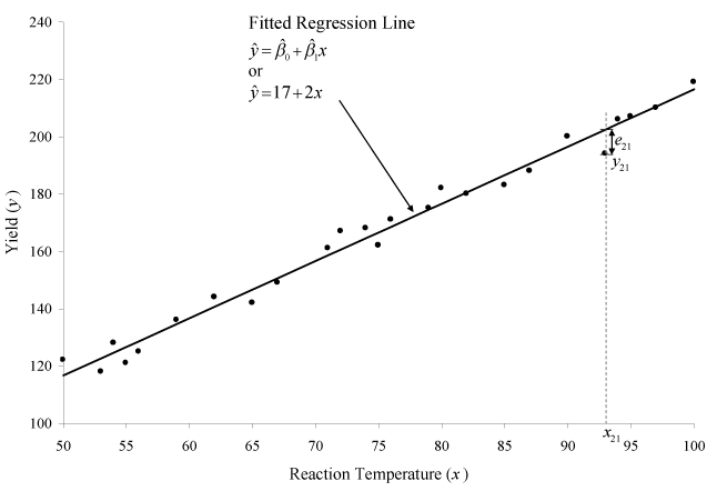
This line is shown in | This line is shown in the figure below. | ||
[[ | [[Image:doe4.4.png|center|637px|Fitted regression line for the data. Also shown is the residual for the 21st observation.|link=]] | ||
Once the fitted regression line is known, the fitted value of <math>Y\,\!</math> corresponding to any observed data point can be calculated. For example, the fitted value corresponding to the 21st observation in the preceding [[Simple_Linear_Regression_Analysis#Simple_Linear_Regression_Analysis| table]] is: | |||
::<math>\begin{align}\hat{y}_{21}= & \hat{\beta}_0 + \hat{\beta}_1 x_{21} \\ | |||
= & (17.0016) + (1.9952) \times 93 \\ | |||
= & 202.6\end{align}\,\!</math> | |||
The observed response at this point is <math>y_{21}=194\,\!</math>. Therefore, the residual at this point is: | |||
: | |||
::<math>\begin{align}e_{21} = & y_{21}-\hat{y}_{21} \\ | |||
= & 194-202.6 \\ | |||
= & -8.6\end{align}\,\!</math> | |||
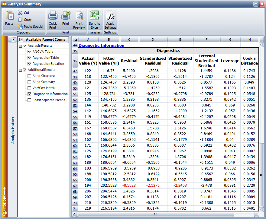
In DOE | In DOE folios, fitted values and residuals can be calculated. The values are shown in the figure below. | ||
[[ | [[Image:doe4_5.png|center|880px|Fitted values and residuals for the data.|link=]] | ||
==Hypothesis Tests in Simple Linear Regression== | |||
The following sections discuss hypothesis tests on the regression coefficients in simple linear regression. These tests can be carried out if it can be assumed that the random error term, <math>\epsilon\,\!</math>, is normally and independently distributed with a mean of zero and variance of <math>\sigma^2\,\!</math>. | |||
===t Tests=== | |||
The <math>t\,\!</math> tests are used to conduct hypothesis tests on the regression coefficients obtained in simple linear regression. A statistic based on the <math>t\,\!</math> distribution is used to test the two-sided hypothesis that the true slope, <math>\beta_1\,\!</math>, equals some constant value, <math>\beta_{1,0}\,\!</math>. The statements for the hypothesis test are expressed as: | |||
::<math>H_0 | ::<math>\begin{align}H_0 & : & \beta_1=\beta_{1,0} \\ | ||
H_1 & : & \beta_{1}\ne\beta_{1,0}\end{align}\,\!</math> | |||
The test statistic used for this test is: | The test statistic used for this test is: | ||
::<math>T_0=\frac{\hat{\beta}_1-\beta_{1,0}}{se(\hat{\beta}_1)}\,\!</math> | |||
where <math>\hat{\beta}_1\,\!</math> is the least square estimate of <math>\beta_1\,\!</math>, and <math>se(\hat{\beta}_1)\,\!</math> is its standard error. The value of <math>se(\hat{\beta}_1)\,\!</math> can be calculated as follows: | |||
:<math>se(\hat{\beta}_1)= \sqrt{\frac{\frac{\displaystyle \sum_{i=1}^n e_i^2}{n-2}}{\displaystyle \sum_{i=1}^n (x_i-\bar{x})^2}}\,\!</math> | |||
The test statistic, <math>T_0\,\!</math> , follows a <math>t\,\!</math> distribution with <math>(n-2)\,\!</math> degrees of freedom, where <math>n\,\!</math> is the total number of observations. The null hypothesis, <math>H_0\,\!</math>, is accepted if the calculated value of the test statistic is such that: | |||
::<math>-t_{\alpha/2,n-2}<T_0<t_{\alpha/2,n-2} </math> | ::<math>-t_{\alpha/2,n-2}<T_0<t_{\alpha/2,n-2}\,\!</math> | ||
where <math>t_{\alpha/2,n-2}\,\!</math> and <math>-t_{\alpha/2,n-2}\,\!</math> are the critical values for the two-sided hypothesis. <math>t_{\alpha/2,n-2}\,\!</math> is the percentile of the <math>t\,\!</math> distribution corresponding to a cumulative probability of <math>(1-\alpha/2)\,\!</math> and <math>\alpha\,\!</math> is the significance level. | |||
If the value of <math>\beta_{1,0}\,\!</math> used is zero, then the hypothesis tests for the significance of regression. In other words, the test indicates if the fitted regression model is of value in explaining variations in the observations or if you are trying to impose a regression model when no true relationship exists between <math>x\,\!</math> and <math>Y\,\!</math>. Failure to reject <math>H_0:\beta_1=0\,\!</math> implies that no linear relationship exists between <math>x\,\!</math> and <math>Y\,\!</math>. This result may be obtained when the scatter plots of against are as shown in (a) of the following figure and (b) of the following figure. (a) represents the case where no model exits for the observed data. In this case you would be trying to fit a regression model to noise or random variation. (b) represents the case where the true relationship between <math>x\,\!</math> and <math>Y\,\!</math> is not linear. (c) and (d) represent the case when <math>H_0:\beta_1=0\,\!</math> is rejected, implying that a model does exist between <math>x\,\!</math> and <math>Y\,\!</math>. (c) represents the case where the linear model is sufficient. In the following figure, (d) represents the case where a higher order model may be needed. | |||
[[Image:doe4.6.png|center|500px|Possible scatter plots of <math>y\,\!</math> against <math>x\,\!</math>. Plots (a) and (b) represent cases when <math>H_0:\beta_1=0\,\!</math> is not rejected. Plots (c) and (d) represent cases when <math>H_0:\beta_1=0\,\!</math> is rejected.|link=]] | |||
A similar procedure can be used to test the hypothesis on the intercept . The test statistic used in this case is: | A similar procedure can be used to test the hypothesis on the intercept. The test statistic used in this case is: | ||
::<math>T_0=\frac{\ | ::<math>T_0=\frac{\hat{\beta}_0-\beta_{0,0}}{se(\hat{\beta}_0)}\,\!</math> | ||
<math>se(\ | where <math>\hat{\beta}_0\,\!</math> is the least square estimate of <math>\beta_0\,\!</math>, and <math>se(\hat{\beta}_0)\,\!</math> is its standard error which is calculated using: | ||
:<math>se(\hat{\beta}_0)= \sqrt{\frac{\displaystyle\sum_{i=1}^n e_i^2}{n-2} \Bigg[ \frac{1}{n}+\frac{\bar{x}^2}{\displaystyle\sum_{i=1}^n (x_i-\bar{x})^2} \Bigg]}\,\!</math> | |||
'''Example''' | |||
The test for the significance of regression for the data in the preceding [[Simple_Linear_Regression_Analysis#Simple_Linear_Regression_Analysis| table]] is illustrated in this example. The test is carried out using the <math>t\,\!</math> test on the coefficient <math>\beta_1\,\!</math>. The hypothesis to be tested is <math>H_0 : \beta_1 = 0\,\!</math>. To calculate the statistic to test <math>H_0\,\!</math>, the estimate, <math>\hat{\beta}_1\,\!</math>, and the standard error, <math>se(\hat{\beta}_1)\,\!</math>, are needed. The value of <math>\hat{\beta}_1\,\!</math> was obtained in [[Simple_Linear_Regression_Analysis#Fitted_Regression_Line|this section]]. The standard error can be calculated as follows: | |||
:<math>\begin{align}se(\hat{\beta}_1) & = \sqrt{\frac{\frac{\displaystyle \sum_{i=1}^n e_i^2}{n-2}}{\displaystyle \sum_{i=1}^n (x_i-\bar{x})^2}} \\ | |||
= & \sqrt{\frac{(371.627/23)}{5679.36}} \\ | |||
= & 0.0533\end{align}\,\!</math> | |||
Then, the test statistic can be calculated using the following equation: | Then, the test statistic can be calculated using the following equation: | ||
The <math>p </math> value corresponding to this statistic based on the <math>t </math> distribution with 23( | ::<math>\begin{align}t_0 & = & \frac{\hat{\beta}_1-\beta_{1,0}}{se(\hat{\beta}_0)} | ||
= & \frac{1.9952-0}{0.0533} | |||
= & 37.4058\end{align}\,\!</math> | |||
The <math>p\,\!</math> value corresponding to this statistic based on the <math>t\,\!</math> distribution with 23 (n-2 = 25-2 = 23) degrees of freedom can be obtained as follows: | |||
::<math>p value = 2 | ::<math>\begin{align}p value = & 2\times (1-P(T\le t_0) \\ | ||
= & 2 \times (1-0.999999) \\ | |||
= & 0\end{align}\,\!</math> | |||
Assuming that the desired significance level is 0.1, since <math>p\,\!</math> value < 0.1, <math>H_0 : \beta_1=0\,\!</math> is rejected indicating that a relation exists between temperature and yield for the data in the preceding [[Simple_Linear_Regression_Analysis#Simple_Linear_Regression_Analysis| table]]. Using this result along with the scatter plot, it can be concluded that the relationship between temperature and yield is linear. | |||
In | In Weibull++ DOE folios, information related to the <math>t\,\!</math> test is displayed in the Regression Information table as shown in the following figure. In this table the <math>t\,\!</math> test for <math>\beta_1\,\!</math> is displayed in the row for the term Temperature because <math>\beta_1\,\!</math> is the coefficient that represents the variable temperature in the regression model. The columns labeled Standard Error, T Value and P Value represent the standard error, the test statistic for the test and the <math>p\,\!</math> value for the <math>t\,\!</math> test, respectively. These values have been calculated for <math>\beta_1\,\!</math> in this example. The Coefficient column represents the estimate of regression coefficients. The Effect column represents values obtained by multiplying the coefficients by a factor of 2. This value is useful in the case of two factor experiments and is explained in [[Two_Level_Factorial_Experiments| Two Level Factorial Experiments]]. Columns Low Confidence and High Confidence represent the limits of the confidence intervals for the regression coefficients and are explained in [[Simple_Linear_Regression_Analysis#Confidence_Interval_on_Regression_Coefficients|Confidence Interval on Regression Coefficients]]. | ||
[[ | [[Image:doe4_7.png|center|826px|Regression results for the data.|link=]] | ||
===Analysis of Variance Approach to Test the Significance of Regression=== | ===Analysis of Variance Approach to Test the Significance of Regression=== | ||
| Line 216: | Line 210: | ||
====Sum of Squares==== | ====Sum of Squares==== | ||
The total variance (i.e. the variance of all of the observed data) is estimated using the observed data. As mentioned in | The total variance (i.e., the variance of all of the observed data) is estimated using the observed data. As mentioned in [[Statistical_Background_on_DOE| Statistical Background]], the variance of a population can be estimated using the sample variance, which is calculated using the following relationship: | ||
::<math>{{s}^{2}}=\frac{\underset{i=1}{\overset{n}{\mathop{\sum }}}\,{{({{y}_{i}}-\bar{y})}^{2}}}{n-1}\,\!</math> | |||
The quantity in the numerator of the previous equation is called the ''sum of squares''. It is the sum of the square of deviations of all the observations, <math>{{y}_{i}}\,\!</math>, from their mean, <math>\bar{y}\,\!</math>. In the context of ANOVA this quantity is called the ''total sum of squares'' (abbreviated <math>S{{S}_{T}}\,\!</math>) because it relates to the total variance of the observations. Thus: | |||
::<math>S{{S}_{T}}=\underset{i=1}{\overset{n}{\mathop \sum }}\,{{({{y}_{i}}-\bar{y})}^{2}}\,\!</math> | |||
The denominator in the relationship of the sample variance is the number of degrees of freedom associated with the sample variance. Therefore, the number of degrees of freedom associated with <math>S{{S}_{T}}\,\!</math>, <math>dof(S{{S}_{T}})\,\!</math>, is <math>n-1\,\!</math>. The sample variance is also referred to as a ''mean square'' because it is obtained by dividing the sum of squares by the respective degrees of freedom. Therefore, the total mean square (abbreviated <math>M{{S}_{T}}\,\!</math>) is: | |||
::<math>M{{S}_{T}}=\frac{S{{S}_{T}}}{dof(S{{S}_{T}})}=\frac{S{{S}_{T}}}{n-1}\,\!</math> | |||
When you attempt to fit a regression model to the observations, you are trying to explain some of the variation of the observations using this model. If the regression model is such that the resulting fitted regression line passes through all of the observations, then you would have a "perfect" model (see (a) of the figure below). In this case the model would explain all of the variability of the observations. Therefore, the model sum of squares (also referred to as the regression sum of squares and abbreviated <math>S{{S}_{R}}\,\!</math>) equals the total sum of squares; i.e., the model explains all of the observed variance: | |||
::<math>S{{S}_{R}}=S{{S}_{T}}\,\!</math> | |||
For the perfect model, the regression sum of squares, <math>S{{S}_{R}}\,\!</math>, equals the total sum of squares, <math>S{{S}_{T}}\,\!</math>, because all estimated values, <math>{{\hat{y}}_{i}}\,\!</math>, will equal the corresponding observations, <math>{{y}_{i}}\,\!</math>. <math>S{{S}_{R}}\,\!</math> can be calculated using a relationship similar to the one for obtaining <math>S{{S}_{T}}\,\!</math> by replacing <math>{{y}_{i}}\,\!</math> by <math>{{\hat{y}}_{i}}\,\!</math> in the relationship of <math>S{{S}_{T}}\,\!</math>. Therefore: | |||
::<math>S{{S}_{R}}=\underset{i=1}{\overset{n}{\mathop \sum }}\,{{({{\hat{y}}_{i}}-\bar{y})}^{2}}\,\!</math> | |||
The | The number of degrees of freedom associated with <math>S{{S}_{R}}\,\!</math> is 1. | ||
Based on the preceding discussion of ANOVA, a perfect regression model exists when the fitted regression line passes through all observed points. However, this is not usually the case, as seen in (b) of the following figure. | |||
[[ | [[Image:doe4.8.png|center|300px|A perfect regression model will pass through all observed data points as shown in (a). Most models are imperfect and do not fit perfectly to all data points as shown in (b).|link=]] | ||
In both of these plots, a number of points do not follow the fitted regression line. This indicates that a part of the total variability of the observed data still remains unexplained. This portion of the total variability or the total sum of squares, that is not explained by the model, is called the ''residual sum of squares'' or the ''error sum of squares'' (abbreviated <math>S{{S}_{E}}\,\!</math>). The deviation for this sum of squares is obtained at each observation in the form of the residuals, <math>{{e}_{i}}\,\!</math>. The error sum of squares can be obtained as the sum of squares of these deviations: | |||
::<math>S{{S}_{E}}=\underset{i=1}{\overset{n}{\mathop \sum }}\,e_{i}^{2}=\underset{i=1}{\overset{n}{\mathop \sum }}\,{{({{y}_{i}}-{{\hat{y}}_{i}})}^{2}}\,\!</math> | |||
The number of degrees of freedom associated with <math>S{{S}_{E}}\,\!</math>, <math>dof(S{{S}_{E}})\,\!</math>, is <math>(n-2)\,\!</math>. | |||
The total variability of the observed data (i.e., total sum of squares, <math>S{{S}_{T}}\,\!</math>) can be written using the portion of the variability explained by the model, <math>S{{S}_{R}}\,\!</math>, and the portion unexplained by the model, <math>S{{S}_{E}}\,\!</math>, as: | |||
::<math>S{{S}_{T}}=S{{S}_{R}}+S{{S}_{E}}\,\!</math> | |||
The above equation is also referred to as the analysis of variance identity and can be expanded as follows: | The above equation is also referred to as the analysis of variance identity and can be expanded as follows: | ||
( | |||
::<math>\underset{i=1}{\overset{n}{\mathop \sum }}\,{{({{y}_{i}}-\bar{y})}^{2}}=\underset{i=1}{\overset{n}{\mathop \sum }}\,{{({{\hat{y}}_{i}}-\bar{y})}^{2}}+\underset{i=1}{\overset{n}{\mathop \sum }}\,{{({{y}_{i}}-{{\hat{y}}_{i}})}^{2}}\,\!</math> | |||
[[Image:doe4.9.png|center|600px|Scatter plots showing the deviations for the sum of squares used in ANOVA. (a) shows deviations for <math>S S_{T}\,\!</math>, (b) shows deviations for <math>S S_{R}\,\!</math>, and (c) shows deviations for <math>S S_{E}\,\!</math>.|link=]] | |||
====Mean Squares==== | |||
As mentioned previously, mean squares are obtained by dividing the sum of squares by the respective degrees of freedom. For example, the error mean square, <math>M{{S}_{E}}\,\!</math>, can be obtained as: | |||
::<math>M{{S}_{E}}=\frac{S{{S}_{E}}}{dof(S{{S}_{E}})}=\frac{S{{S}_{E}}}{n-2}\,\!</math> | |||
The error mean square is an estimate of the variance, <math>{{\sigma }^{2}}\,\!</math>, of the random error term, <math>\epsilon\,\!</math>, and can be written as: | |||
= | ::<math>{{\hat{\sigma }}^{2}}=\frac{S{{S}_{E}}}{n-2}\,\!</math> | ||
Similarly, the regression mean square, <math>M{{S}_{R}}\,\!</math>, can be obtained by dividing the regression sum of squares by the respective degrees of freedom as follows: | |||
::<math>M{{S}_{R}}=\frac{S{{S}_{R}}}{dof(S{{S}_{R}})}=\frac{S{{S}_{R}}}{1}\,\!</math> | |||
====F Test==== | ====F Test==== | ||
To test the hypothesis , the statistic used is based on the | To test the hypothesis <math>{{H}_{0}}:{{\beta }_{1}}=0\,\!</math>, the statistic used is based on the <math>F\,\!</math> distribution. It can be shown that if the null hypothesis <math>{{H}_{0}}\,\!</math> is true, then the statistic: | ||
::<math>{{F}_{0}}=\frac{M{{S}_{R}}}{M{{S}_{E}}}=\frac{S{{S}_{R}}/1}{S{{S}_{E}}/(n-2)}\,\!</math> | |||
follows the <math>F\,\!</math> distribution with <math>1\,\!</math> degree of freedom in the numerator and <math>(n-2)\,\!</math> degrees of freedom in the denominator. <math>{{H}_{0}}\,\!</math> is rejected if the calculated statistic, <math>{{F}_{0}}\,\!</math>, is such that: | |||
::<math>{{F}_{0}}>{{f}_{\alpha ,1,n-2}}\,\!</math> | |||
where <math>{{f}_{\alpha ,1,n-2}}\,\!</math> is the percentile of the <math>F\,\!</math> distribution corresponding to a cumulative probability of (<math>1-\alpha\,\!</math>) and <math>\alpha\,\!</math> is the significance level. | |||
'''Example''' | |||
The analysis of variance approach to test the significance of regression can be applied to the yield data in the preceding [[Simple_Linear_Regression_Analysis#Simple_Linear_Regression_Analysis| table]]. To calculate the statistic, <math>{{F}_{0}}\,\!</math>, for the test, the sum of squares have to be obtained. The sum of squares can be calculated as shown next. | |||
The total sum of squares can be calculated as: | The total sum of squares can be calculated as: | ||
::<math>\begin{align} | |||
S{{S}_{T}}= & \underset{i=1}{\overset{n}{\mathop \sum }}\,{{({{y}_{i}}-\bar{y})}^{2}} \\ | |||
= & \underset{i=1}{\overset{25}{\mathop \sum }}\,{{({{y}_{i}}-166.32)}^{2}} \\ | |||
= & 22979.44 | |||
\end{align}\,\!</math> | |||
The regression sum of squares can be calculated as: | The regression sum of squares can be calculated as: | ||
::<math>\begin{align} | |||
S{{S}_{R}}= & \underset{i=1}{\overset{n}{\mathop \sum }}\,{{({{{\hat{y}}}_{i}}-\bar{y})}^{2}} \\ | |||
= & \underset{i=1}{\overset{25}{\mathop \sum }}\,{{({{{\hat{y}}}_{i}}-166.32)}^{2}} \\ | |||
= & 22607.81 | |||
\end{align}\,\!</math> | |||
| Line 308: | Line 333: | ||
Knowing the sum of squares, the statistic to test | ::<math>\begin{align} | ||
S{{S}_{E}}= & \underset{i=1}{\overset{n}{\mathop \sum }}\,{{({{y}_{i}}-{{{\hat{y}}}_{i}})}^{2}} \\ | |||
= & \underset{i=1}{\overset{25}{\mathop \sum }}\,{{({{y}_{i}}-{{{\hat{y}}}_{i}})}^{2}} \\ | |||
= & 371.63 | |||
\end{align}\,\!</math> | |||
Knowing the sum of squares, the statistic to test <math>{{H}_{0}}:{{\beta }_{1}}=0\,\!</math> can be calculated as follows: | |||
::<math>\begin{align} | |||
{{f}_{0}}=& \frac{M{{S}_{R}}}{M{{S}_{E}}} \\ | |||
= & \frac{S{{S}_{R}}/1}{S{{S}_{E}}/(n-2)} \\ | |||
= & \frac{22607.81/1}{371.63/(25-2)} \\ | |||
= & 1399.20 | |||
\end{align}\,\!</math> | |||
The critical value at a significance level of 0.1 is <math>{{f}_{0.05,1,23}}=2.937\,\!</math>. Since <math>{{f}_{0}}>{{f}_{\alpha ,1,n-2}}\,\!</math>, <math>{{H}_{0}}:{{\beta }_{1}}=0\,\!</math> is rejected and it is concluded that <math>{{\beta }_{1}}\,\!</math> is not zero. Alternatively, the <math>p\,\!</math> value can also be used. The <math>p\,\!</math> value corresponding to the test statistic, <math>{{f}_{0}}\,\!</math>, based on the <math>F\,\!</math> distribution with one degree of freedom in the numerator and 23 degrees of freedom in the denominator is: | |||
::<math>\begin{align} | |||
p\text{ }value= & 1-P(F\le {{f}_{0}}) \\ | |||
= & 1-0.999999 \\ | |||
= & 4.17E-22 | |||
\end{align}\,\!</math> | |||
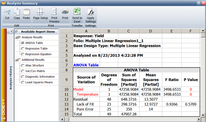
Assuming that the desired significance is 0.1, since the | Assuming that the desired significance is 0.1, since the <math>p\,\!</math> value < 0.1, then <math>{{H}_{0}}:{{\beta }_{1}}=0\,\!</math> is rejected, implying that a relation does exist between temperature and yield for the data in the preceding [[Simple_Linear_Regression_Analysis#Simple_Linear_Regression_Analysis| table]]. Using this result along with the scatter plot of the above [[Simple_Linear_Regression_Analysis#Simple_Linear_Regression_Analysis| figure]], it can be concluded that the relationship that exists between temperature and yield is linear. This result is displayed in the ANOVA table as shown in the following figure. Note that this is the same result that was obtained from the <math>t\,\!</math> test in the section [[Simple_Linear_Regression_Analysis#Tests|t Tests]]. The ANOVA and Regression Information tables in Weibull++ DOE folios represent two different ways to test for the significance of the regression model. In the case of multiple linear regression models these tables are expanded to allow tests on individual variables used in the model. This is done using extra sum of squares. Multiple linear regression models and the application of extra sum of squares in the analysis of these models are discussed in [[Multiple_Linear_Regression_Analysis| Multiple Linear Regression Analysis]]. | ||
[[ | [[Image:doe4_10.png|center|747px| ANOVA table for the data.|link=]] | ||
==Confidence Intervals in Simple Linear Regression== | ==Confidence Intervals in Simple Linear Regression== | ||
A confidence interval represents a closed interval where a certain percentage of the population is likely to lie. For example, a 90% confidence interval with a lower limit of | A confidence interval represents a closed interval where a certain percentage of the population is likely to lie. For example, a 90% confidence interval with a lower limit of <math>A\,\!</math> and an upper limit of <math>B\,\!</math> implies that 90% of the population lies between the values of <math>A\,\!</math> and <math>B\,\!</math>. Out of the remaining 10% of the population, 5% is less than <math>A\,\!</math> and 5% is greater than <math>B\,\!</math>. (For details refer to the Life data analysis reference.) This section discusses confidence intervals used in simple linear regression analysis. | ||
===Confidence Interval on Regression Coefficients=== | ===Confidence Interval on Regression Coefficients=== | ||
A 100() percent confidence interval on | A 100 (<math>1-\alpha\,\!</math>) percent confidence interval on <math>{{\beta }_{1}}\,\!</math> is obtained as follows: | ||
( | |||
::<math>{{\hat{\beta }}_{1}}\pm {{t}_{\alpha /2,n-2}}\cdot se({{\hat{\beta }}_{1}})\,\!</math> | |||
Similarly, a 100 (<math>1-\alpha\,\!</math>) percent confidence interval on <math>{{\beta }_{0}}\,\!</math> is obtained as: | |||
::<math>{{\hat{\beta }}_{0}}\pm {{t}_{\alpha /2,n-2}}\cdot se({{\hat{\beta }}_{0}})\,\!</math> | |||
===Confidence Interval on Fitted Values=== | ===Confidence Interval on Fitted Values=== | ||
A 100() percent confidence interval on any fitted value, , is obtained as follows: | A 100 (<math>1-\alpha\,\!</math>) percent confidence interval on any fitted value, <math>{{\hat{y}}_{i}}\,\!</math>, is obtained as follows: | ||
( | |||
::<math>{{\hat{y}}_{i}}\pm {{t}_{\alpha /2,n-2}}\sqrt{{{{\hat{\sigma }}}^{2}}\left[ \frac{1}{n}+\frac{{{({{x}_{i}}-\bar{x})}^{2}}}{\underset{i=1}{\overset{n}{\mathop \sum }}\,{{({{x}_{i}}-\bar{x})}^{2}}} \right]}\,\!</math> | |||
It can be seen that the width of the confidence interval depends on the value of <math>{{x}_{i}}\,\!</math> and will be a minimum at <math>{{x}_{i}}=\bar{x}\,\!</math> and will widen as <math>\left| {{x}_{i}}-\bar{x} \right|\,\!</math> increases. | |||
===Confidence Interval on New Observations=== | ===Confidence Interval on New Observations=== | ||
For the data in | For the data in the preceding [[Simple_Linear_Regression_Analysis#Simple_Linear_Regression_Analysis| table]], assume that a new value of the yield is observed after the regression model is fit to the data. This new observation is independent of the observations used to obtain the regression model. If <math>{{x}_{p}}\,\!</math> is the level of the temperature at which the new observation was taken, then the estimate for this new value based on the fitted regression model is: | ||
::<math>\begin{align} | |||
{{{\hat{y}}}_{p}}= & {{{\hat{\beta }}}_{0}}+{{{\hat{\beta }}}_{1}}{{x}_{p}} \\ | |||
= & 17.0016+1.9952\times {{x}_{p}} \\ | |||
\end{align}\,\!</math> | |||
'''Example | If a confidence interval needs to be obtained on <math>{{\hat{y}}_{p}}\,\!</math>, then this interval should include both the error from the fitted model and the error associated with future observations. This is because <math>{{\hat{y}}_{p}}\,\!</math> represents the estimate for a value of <math>Y\,\!</math> that was not used to obtain the regression model. The confidence interval on <math>{{\hat{y}}_{p}}\,\!</math> is referred to as the ''prediction interval''. A 100 (<math>1-\alpha\,\!</math>) percent prediction interval on a new observation is obtained as follows: | ||
::<math>{{\hat{y}}_{p}}\pm {{t}_{\alpha /2,n-2}}\sqrt{{{{\hat{\sigma }}}^{2}}\left[ 1+\frac{1}{n}+\frac{{{({{x}_{p}}-\bar{x})}^{2}}}{\underset{i=1}{\overset{n}{\mathop \sum }}\,{{({{x}_{p}}-\bar{x})}^{2}}} \right]}\,\!</math> | |||
'''Example''' | |||
To illustrate the calculation of confidence intervals, the 95% confidence intervals on the response at <math>x=93\,\!</math> for the data in the preceding [[Simple_Linear_Regression_Analysis#Simple_Linear_Regression_Analysis| table]] is obtained in this example. A 95% prediction interval is also obtained assuming that a new observation for the yield was made at <math>x=91\,\!</math>. | |||
The fitted value, <math>{{\hat{y}}_{i}}\,\!</math>, corresponding to <math>x=93\,\!</math> is: | |||
::<math>\begin{align} | |||
{{{\hat{y}}}_{21}}= & {{{\hat{\beta }}}_{0}}+{{{\hat{\beta }}}_{1}}{{x}_{21}} \\ | |||
= & 17.0016+1.9952\times 93 \\ | |||
= & 202.6 | |||
\end{align}\,\!</math> | |||
The fitted value, , | The 95% confidence interval <math>(\alpha =0.05)\,\!</math> on the fitted value, <math>{{\hat{y}}_{21}}=202.6\,\!</math>, is: | ||
::<math>\begin{align} | |||
= & {{{\hat{y}}}_{i}}\pm {{t}_{\alpha /2,n-2}}\sqrt{{{{\hat{\sigma }}}^{2}}\left[ \frac{1}{n}+\frac{{{({{x}_{i}}-\bar{x})}^{2}}}{\underset{i=1}{\overset{n}{\mathop \sum }}\,{{({{x}_{i}}-\bar{x})}^{2}}} \right]} \\ | |||
= & 202.6\pm {{t}_{0.025,23}}\sqrt{M{{S}_{E}}\left[ \frac{1}{25}+\frac{{{(93-74.84)}^{2}}}{5679.36} \right]} \\ | |||
= & 202.6\pm 2.069\sqrt{16.16\left[ \frac{1}{25}+\frac{{{(93-74.84)}^{2}}}{5679.36} \right]} \\ | |||
= & 202.6\pm 2.602 | |||
\end{align}\,\!</math> | |||
The 95% limits on | The 95% limits on <math>{{\hat{y}}_{21}}\,\!</math> are 199.95 and 205.2, respectively. | ||
The estimated value based on the fitted regression model for the new observation at <math>x=91\,\!</math> is: | |||
::<math>\begin{align} | |||
{{{\hat{y}}}_{p}}= & {{{\hat{\beta }}}_{0}}+{{{\hat{\beta }}}_{1}}{{x}_{p}} \\ | |||
= & 17.0016+1.9952\times 91 \\ | |||
= & 198.6 | |||
\end{align}\,\!</math> | |||
The 95% prediction interval on | The 95% prediction interval on <math>{{\hat{y}}_{p}}=198.6\,\!</math> is: | ||
::<math>\begin{align} | |||
= & {{{\hat{y}}}_{p}}\pm {{t}_{\alpha /2,n-2}}\sqrt{{{{\hat{\sigma }}}^{2}}\left[ 1+\frac{1}{n}+\frac{{{({{x}_{p}}-\bar{x})}^{2}}}{\underset{i=1}{\overset{n}{\mathop \sum }}\,{{({{x}_{p}}-\bar{x})}^{2}}} \right]} \\ | |||
= & 198.6\pm {{t}_{0.025,23}}\sqrt{M{{S}_{E}}\left[ 1+\frac{1}{25}+\frac{{{(93-74.84)}^{2}}}{5679.36} \right]} \\ | |||
= & 198.6\pm 2.069\sqrt{16.16\left[ 1+\frac{1}{25}+\frac{{{(93-74.84)}^{2}}}{5679.36} \right]} \\ | |||
= & 198.6\pm 2.069\times 4.1889 \\ | |||
= & 198.6\pm 8.67 | |||
\end{align}\,\!</math> | |||
The 95% limits on <math>{{\hat{y}}_{p}}\,\!</math> are 189.9 and 207.2, respectively. In Weibull++ DOE folios, confidence and prediction intervals can be calculated from the control panel. The prediction interval values calculated in this example are shown in the figure below as Low Prediction Interval and High Prediction Interval, respectively. The columns labeled Mean Predicted and Standard Error represent the values of <math>{{\hat{y}}_{p}}\,\!</math> and the standard error used in the calculations. | |||
[[Image:doe4_11.png|center|786px|Calculation of prediction intervals in Weibull++.|link=]] | |||
==Measures of Model Adequacy== | ==Measures of Model Adequacy== | ||
It is important to analyze the regression model before inferences based on the model are undertaken. The following sections present some techniques that can be used to check the appropriateness of the model for the given data. These techniques help to determine if any of the model assumptions have been violated. | It is important to analyze the regression model before inferences based on the model are undertaken. The following sections present some techniques that can be used to check the appropriateness of the model for the given data. These techniques help to determine if any of the model assumptions have been violated. | ||
===Coefficient of Determination (<math>R^2 </math>)=== | |||
The coefficient of determination is a measure of the amount of variability in the data accounted for by the regression model. As mentioned previously, the total variability of the data is measured by the total sum of squares, <math>SS_T\,\!</math>. The amount of this variability explained by the regression model is the regression sum of squares, <math>SS_R\,\!</math>. The coefficient of determination is the ratio of the regression sum of squares to the total sum of squares. | |||
::<math>R^2 = \frac{SS_R}{SS_T}\,\!</math> | |||
= | <math>R^2\,\!</math> can take on values between 0 and 1 since <math>R^2 = \frac{SS_R}{SS_T}\,\!</math> . For the yield data example, <math>R^2\,\!</math> can be calculated as: | ||
::<math>\begin{align} | |||
{{R}^{2}}= & \frac{S{{S}_{R}}}{S{{S}_{T}}} \\ | |||
= & \frac{22607.81}{22979.44} \\ | |||
= & 0.98 | |||
\end{align}\,\!</math> | |||
Therefore, 98% of the variability in the yield data is explained by the regression model, indicating a very good fit of the model. It may appear that larger values of <math>{{R}^{2}}\,\!</math> indicate a better fitting regression model. However, <math>{{R}^{2}}\,\!</math> should be used cautiously as this is not always the case. The value of <math>{{R}^{2}}\,\!</math> increases as more terms are added to the model, even if the new term does not contribute significantly to the model. Therefore, an increase in the value of <math>{{R}^{2}}\,\!</math> cannot be taken as a sign to conclude that the new model is superior to the older model. Adding a new term may make the regression model worse if the error mean square, <math>M{{S}_{E}}\,\!</math>, for the new model is larger than the <math>M{{S}_{E}}\,\!</math> of the older model, even though the new model will show an increased value of <math>{{R}^{2}}\,\!</math>. In the results obtained from the DOE folio, <math>{{R}^{2}}\,\!</math> is displayed as R-sq under the ANOVA table (as shown in the figure below), which displays the complete analysis sheet for the data in the preceding [[Simple_Linear_Regression_Analysis#Simple_Linear_Regression_Analysis| table]]. | |||
The other values displayed with are S, R-sq(adj), PRESS and R-sq(pred). These values measure different aspects of the adequacy of the regression model. For example, the value of S is the square root of the error mean square, <math>MS_E\,\!</math>, and represents the "standard error of the model." A lower value of S indicates a better fitting model. The values of S, R-sq and R-sq(adj) indicate how well the model fits the observed data. The values of PRESS and R-sq(pred) are indicators of how well the regression model predicts new observations. R-sq(adj), PRESS and R-sq(pred) are explained in [[Multiple Linear Regression Analysis]]. | |||
[[Image:doe4_12.png|center|874px|Complete analysis for the data.|link=]] | |||
===Residual Analysis=== | |||
In the simple linear regression model the true error terms, <math>{{\epsilon }_{i}}\,\!</math>, are never known. The residuals, <math>{{e}_{i}}\,\!</math>, may be thought of as the observed error terms that are similar to the true error terms. Since the true error terms, <math>{{\epsilon }_{i}}\,\!</math>, are assumed to be normally distributed with a mean of zero and a variance of <math>{{\sigma }^{2}}\,\!</math>, in a good model the observed error terms (i.e., the residuals, <math>{{e}_{i}}\,\!</math>) should also follow these assumptions. Thus the residuals in the simple linear regression should be normally distributed with a mean of zero and a constant variance of <math>{{\sigma }^{2}}\,\!</math>. Residuals are usually plotted against the fitted values, <math>{{\hat{y}}_{i}}\,\!</math>, against the predictor variable values, <math>{{x}_{i}}\,\!</math>, and against time or run-order sequence, in addition to the normal probability plot. Plots of residuals are used to check for the following: | |||
:1. Residuals follow the normal distribution. | |||
:2. Residuals have a constant variance. | |||
:3. Regression function is linear. | |||
:4. A pattern does not exist when residuals are plotted in a time or run-order sequence. | |||
:5. There are no outliers. | |||
Examples of residual plots are shown in the following figure. (a) is a satisfactory plot with the residuals falling in a horizontal band with no systematic pattern. Such a plot indicates an appropriate regression model. (b) shows residuals falling in a funnel shape. Such a plot indicates increase in variance of residuals and the assumption of constant variance is violated here. Transformation on <math>Y\,\!</math> may be helpful in this case (see [[Simple_Linear_Regression_Analysis#Transformations| Transformations]]). If the residuals follow the pattern of (c) or (d), then this is an indication that the linear regression model is not adequate. Addition of higher order terms to the regression model or transformation on <math>x\,\!</math> or <math>Y\,\!</math> may be required in such cases. A plot of residuals may also show a pattern as seen in (e), indicating that the residuals increase (or decrease) as the run order sequence or time progresses. This may be due to factors such as operator-learning or instrument-creep and should be investigated further. | |||
[[Image:doe4.13.png|center|550px|Possible residual plots (against fitted values, time or run-order) that can be obtained from simple linear regression analysis.|link=]] | |||
'''Example''' | |||
Residual plots for the data of the preceding [[Simple_Linear_Regression_Analysis#Simple_Linear_Regression_Analysis| table]] are shown in the following figures. One of the following figures is the normal probability plot. It can be observed that the residuals follow the normal distribution and the assumption of normality is valid here. In one of the following figures the residuals are plotted against the fitted values, <math>{{\hat{y}}_{i}}\,\!</math>, and in one of the following figures the residuals are plotted against the run order. Both of these plots show that the 21st observation seems to be an outlier. Further investigations are needed to study the cause of this outlier. | |||
[[Image:doe4_14.png|center|650px|Normal probability plot of residuals for the data.|link=]] | |||
[[ | |||
[[Image:doe4_15.png|center|650px|Plot of residuals against fitted values for the data.|link=]] | |||
[[Image:doe4_16.png|center|650px|Plot of residuals against run order for the data.|link=]] | |||
===Lack-of-Fit Test=== | |||
As mentioned in [[Simple_Linear_Regression_Analysis#Analysis_of_Variance_Approach_to_Test_the_Significance_of_Regression| Analysis of Variance Approach]], ANOVA, a perfect regression model results in a fitted line that passes exactly through all observed data points. This perfect model will give us a zero error sum of squares (<math>S{{S}_{E}}=0\,\!</math>). Thus, no error exists for the perfect model. However, if you record the response values for the same values of <math>{{x}_{i}}\,\!</math> for a second time, in conditions maintained as strictly identical as possible to the first time, observations from the second time will not all fall along the perfect model. The deviations in observations recorded for the second time constitute the "purely" random variation or noise. The sum of squares due to pure error (abbreviated <math>S{{S}_{PE}}\,\!</math>) quantifies these variations. <math>S{{S}_{PE}}\,\!</math> is calculated by taking repeated observations at some or all values of <math>{{x}_{i}}\,\!</math> and adding up the square of deviations at each level of <math>x\,\!</math> using the respective repeated observations at that <math>x\,\!</math> value. | |||
Assume that there are <math>n\,\!</math> levels of <math>x\,\!</math> and <math>{{m}_{i}}\,\!</math> repeated observations are taken at each <math>i\,\!</math> the level. The data is collected as shown next: | |||
1. | ::<math>\begin{align} | ||
& {{y}_{11}},{{y}_{12}},....,{{y}_{1{{m}_{1}}}}\text{ repeated observations at }{{x}_{1}} \\ | |||
& {{y}_{21}},{{y}_{22}},....,{{y}_{2{{m}_{2}}}}\text{ repeated observations at }{{x}_{2}} \\ | |||
& ... \\ | |||
& {{y}_{i1}},{{y}_{i2}},....,{{y}_{i{{m}_{i}}}}\text{ repeated observations at }{{x}_{i}} \\ | |||
& ... \\ | |||
& {{y}_{n1}},{{y}_{n2}},....,{{y}_{n{{m}_{n}}}}\text{ repeated observations at }{{x}_{n}} | |||
\end{align}\,\!</math> | |||
The sum of squares of the deviations from the mean of the observations at <math>i\,\!</math> the level of <math>x\,\!</math>, <math>{{x}_{i}}\,\!</math>, can be calculated as: | |||
::<math>\underset{j=1}{\overset{{{m}_{i}}}{\mathop \sum }}\,{{({{y}_{ij}}-{{\bar{y}}_{i}})}^{2}}\,\!</math> | |||
where <math>{{\bar{y}}_{i}}\,\!</math> is the mean of the <math>{{m}_{i}}\,\!</math> repeated observations corresponding to <math>{{x}_{i}}\,\!</math> (<math>{{\bar{y}}_{i}}=(1/{{m}_{i}})\mathop{}_{j=1}^{{{m}_{i}}}{{y}_{ij}}\,\!</math>). The number of degrees of freedom for these deviations is (<math>{{m}_{i}}-1\,\!</math> ) as there are <math>{{m}_{i}}\,\!</math> observations at <math>i\,\!</math> the level of <math>x\,\!</math> but one degree of freedom is lost in calculating the mean, <math>{{\bar{y}}_{i}}\,\!</math>. | |||
The total sum of square deviations (or <math>S{{S}_{PE}}\,\!</math>) for all levels of <math>x\,\!</math> can be obtained by summing the deviations for all <math>{{x}_{i}}\,\!</math> as shown next: | |||
::<math>S{{S}_{PE}}=\underset{i=1}{\overset{n}{\mathop \sum }}\,\underset{j=1}{\overset{{{m}_{i}}}{\mathop \sum }}\,{{({{y}_{ij}}-{{\bar{y}}_{i}})}^{2}}\,\!</math> | |||
The total number of degrees of freedom associated with <math>S{{S}_{PE}}\,\!</math> is: | |||
::<math>\begin{align} | |||
= & \underset{i=1}{\overset{n}{\mathop \sum }}\,({{m}_{i}}-1) \\ | |||
= & \underset{i=1}{\overset{n}{\mathop \sum }}\,{{m}_{i}}-n | |||
\end{align}\,\!</math> | |||
If all <math>{{m}_{i}}=m\,\!</math>, (i.e., <math>m\,\!</math> repeated observations are taken at all levels of <math>x\,\!</math>), then <math>\mathop{}_{i=1}^{n}{{m}_{i}}=nm\,\!</math> and the degrees of freedom associated with <math>S{{S}_{PE}}\,\!</math> are: | |||
::<math>=nm-n\,\!</math> | |||
The corresponding mean square in this case will be: | |||
::<math>M{{S}_{PE}}=\frac{S{{S}_{PE}}}{nm-n}\,\!</math> | |||
When repeated observations are used for a perfect regression model, the sum of squares due to pure error, <math>S{{S}_{PE}}\,\!</math>, is also considered as the error sum of squares, <math>S{{S}_{E}}\,\!</math>. For the case when repeated observations are used with imperfect regression models, there are two components of the error sum of squares, <math>S{{S}_{E}}\,\!</math>. One portion is the pure error due to the repeated observations. The other portion is the error that represents variation not captured because of the imperfect model. The second portion is termed as the sum of squares due to lack-of-fit (abbreviated <math>S{{S}_{LOF}}\,\!</math>) to point to the deficiency in fit due to departure from the perfect-fit model. Thus, for an imperfect regression model: | |||
::<math>S{{S}_{E}}=S{{S}_{PE}}+S{{S}_{LOF}}\,\!</math> | |||
Knowing <math>S{{S}_{E}}\,\!</math> and <math>S{{S}_{PE}}\,\!</math>, the previous equation can be used to obtain <math>S{{S}_{LOF}}\,\!</math>: | |||
::<math>S{{S}_{LOF}}=S{{S}_{E}}-S{{S}_{PE}}\,\!</math> | |||
The degrees of freedom associated with <math>S{{S}_{LOF}}\,\!</math> can be obtained in a similar manner using subtraction. For the case when <math>m\,\!</math> repeated observations are taken at all levels of <math>x\,\!</math>, the number of degrees of freedom associated with <math>S{{S}_{PE}}\,\!</math> is: | |||
::<math>dof(S{{S}_{PE}})=nm-n\,\!</math> | |||
( | |||
Since there are <math>nm\,\!</math> total observations, the number of degrees of freedom associated with <math>S{{S}_{E}}\,\!</math> is: | |||
::<math>dof(S{{S}_{E}})=nm-2\,\!</math> | |||
Therefore, the number of degrees of freedom associated with <math>S{{S}_{LOF}}\,\!</math> is: | |||
::<math>\begin{align} | |||
= & dof(S{{S}_{E}})-dof(S{{S}_{PE}}) \\ | |||
= & (nm-2)-(nm-n) \\ | |||
= & n-2 | |||
\end{align}\,\!</math> | |||
The corresponding mean square, <math>M{{S}_{LOF}}\,\!</math>, can now be obtained as: | |||
::<math>M{{S}_{LOF}}=\frac{S{{S}_{LOF}}}{n-2}\,\!</math> | |||
The magnitude of <math>S{{S}_{LOF}}\,\!</math> or <math>M{{S}_{LOF}}\,\!</math> will provide an indication of how far the regression model is from the perfect model. An <math>F\,\!</math> test exists to examine the lack-of-fit at a particular significance level. The quantity <math>M{{S}_{LOF}}/M{{S}_{PE}}\,\!</math> follows an <math>F\,\!</math> distribution with <math>(n-2)\,\!</math> degrees of freedom in the numerator and <math>(nm-n)\,\!</math> degrees of freedom in the denominator when all <math>{{m}_{i}}\,\!</math> equal <math>m\,\!</math>. The test statistic for the lack-of-fit test is: | |||
::<math>{{F}_{0}}=\frac{M{{S}_{LOF}}}{M{{S}_{PE}}}\,\!</math> | |||
If the critical value <math>{{f}_{\alpha ,n-2,mn-n}}\,\!</math> is such that: | |||
::<math>{{F}_{0}}>{{f}_{\alpha ,n-2,nm-n}}\,\!</math> | |||
it will lead to the rejection of the hypothesis that the model adequately fits the data. | it will lead to the rejection of the hypothesis that the model adequately fits the data. | ||
'''Example''' | |||
Assume that a second set of observations are taken for the yield data of | Assume that a second set of observations are taken for the yield data of the preceding [http://reliawiki.org/index.php/Simple_Linear_Regression_Analysis#Simple_Linear_Regression_Analysis| table]. The resulting observations are recorded in the following table. To conduct a lack-of-fit test on this data, the statistic <math>{{F}_{0}}=M{{S}_{LOF}}/M{{S}_{PE}}\,\!</math>, can be calculated as shown next. | ||
[[Image:doet4.2.png|center|436px|Yield data from the first and second observation sets for the chemical process example in the Introduction.|link=]] | |||
[[ | |||
'''Calculation of Least Square Estimates''' | '''Calculation of Least Square Estimates''' | ||
Knowing | The parameters of the fitted regression model can be obtained as: | ||
::<math>\begin{align} | |||
{{{\hat{\beta }}}_{1}} = & \frac{\underset{i=1}{\overset{50}{\mathop \sum }}\,{{y}_{i}}{{x}_{i}}-\frac{\left( \underset{i=1}{\overset{50}{\mathop \sum }}\,{{y}_{i}} \right)\left( \underset{i=1}{\overset{50}{\mathop \sum }}\,{{x}_{i}} \right)}{50}}{\underset{i=1}{\overset{50}{\mathop \sum }}\,{{({{x}_{i}}-\bar{x})}^{2}}} \\ | |||
= & \frac{648532-\frac{8356\times 3742}{50}}{11358.72} \\ | |||
= & 2.04 \end{align}\,\!</math> | |||
::<math>\begin{align} | |||
{{{\hat{\beta }}}_{0}}= & \bar{y}-{{{\hat{\beta }}}_{1}}\bar{x} \\ | |||
= & 167.12-2.04\times 74.84 \\ | |||
= & 14.47 | |||
\end{align}\,\!</math> | |||
Knowing <math>{{\hat{\beta }}_{1}}\,\!</math> and <math>{{\hat{\beta }}_{0}}\,\!</math>, the fitted values, <math>{{\hat{y}}_{i}}\,\!</math>, can be calculated. | |||
'''Calculation of the Sum of Squares''' | '''Calculation of the Sum of Squares''' | ||
| Line 562: | Line 665: | ||
::<math>\begin{align} | |||
S{{S}_{T}} = & \underset{i=1}{\overset{50}{\mathop \sum }}\,{{({{y}_{i}}-\bar{y})}^{2}} \\ | |||
= & 47907.28 \end{align}\,\!</math> | |||
::<math>\begin{align} | |||
S{{S}_{R}} = & \underset{i=1}{\overset{50}{\mathop \sum }}\,{{({{{\hat{y}}}_{i}}-\bar{y})}^{2}} \\ | |||
= & 47258.91 \end{align} | |||
\,\!</math> | |||
::<math>\begin{align} | |||
S{{S}_{E}} = & \underset{i=1}{\overset{50}{\mathop \sum }}\,{{({{y}_{i}}-{{{\hat{y}}}_{i}})}^{2}} \\ | |||
= & 648.37 \end{align} | |||
\,\!</math> | |||
'''Calculation of <math>M{{S}_{LOF}}\,\!</math>''' | |||
The error sum of squares, <math>S{{S}_{E}}\,\!</math>, can now be split into the sum of squares due to pure error, <math>S{{S}_{PE}}\,\!</math>, and the sum of squares due to lack-of-fit, <math>S{{S}_{LOF}}\,\!</math>. <math>S{{S}_{PE}}\,\!</math> can be calculated as follows considering that in this example <math>n=25\,\!</math> and <math>m=2\,\!</math>: | |||
::<math> | |||
Similarly, the number of degrees of freedom associated with | \begin{align} | ||
S{{S}_{PE}} & = \underset{i=1}{\overset{n}{\mathop \sum }}\,\underset{j=1}{\overset{{{m}_{i}}}{\mathop \sum }}\,{{({{y}_{ij}}-{{{\bar{y}}}_{i}})}^{2}} \\ | |||
& = \underset{i=1}{\overset{25}{\mathop \sum }}\,\underset{j=1}{\overset{2}{\mathop \sum }}\,{{({{y}_{ij}}-{{{\bar{y}}}_{i}})}^{2}} \\ | |||
& = 350 | |||
\end{align}\,\! | |||
</math> | |||
The number of degrees of freedom associated with <math>S{{S}_{PE}}\,\!</math> is: | |||
::<math>\begin{align} | |||
dof(S{{S}_{PE}}) & = nm-n \\ | |||
& = 25\times 2-25 \\ | |||
& = 25 | |||
\end{align}\,\!</math> | |||
The corresponding mean square, <math>M{{S}_{PE}}\,\!</math>, can now be obtained as: | |||
::<math>\begin{align} | |||
M{{S}_{PE}} & = \frac{S{{S}_{PE}}}{dof(S{{S}_{PE}})} \\ | |||
& = \frac{350}{25} \\ | |||
& = 14 | |||
\end{align}\,\!</math> | |||
<math>S{{S}_{LOF}}\,\!</math> can be obtained by subtraction from <math>S{{S}_{E}}\,\!</math> as: | |||
::<math>\begin{align} | |||
S{{S}_{LOF}} & = S{{S}_{E}}-S{{S}_{PE}} \\ | |||
& = 648.37-350 \\ | |||
& = 298.37 | |||
\end{align}\,\!</math> | |||
Similarly, the number of degrees of freedom associated with <math>S{{S}_{LOF}}\,\!</math> is: | |||
::<math>\begin{align} | |||
dof(S{{S}_{LOF}}) & = dof(S{{S}_{E}})-dof(S{{S}_{PE}}) \\ | |||
& = (nm-2)-(nm-n) \\ | |||
& = 23 | |||
\end{align}\,\!</math> | |||
The lack-of-fit mean square is: | The lack-of-fit mean square is: | ||
::<math>\begin{align} | |||
M{{S}_{LOF}} & = \frac{M{{S}_{LOF}}}{dof(M{{S}_{LOF}})} \\ | |||
& = \frac{298.37}{23} \\ | |||
& = 12.97 | |||
\end{align}\,\!</math> | |||
'''Calculation of the Test Statistic''' | '''Calculation of the Test Statistic''' | ||
The test statistic for the lack-of-fit test can now be calculated as: | The test statistic for the lack-of-fit test can now be calculated as: | ||
::<math>\begin{align} | |||
{{f}_{0}} & = \frac{M{{S}_{LOF}}}{M{{S}_{PE}}} \\ | |||
& = \frac{12.97}{14} \\ | |||
& = 0.93 | |||
\end{align}\,\!</math> | |||
| Line 590: | Line 765: | ||
::<math>{{f}_{0.05,23,25}}=1.97\,\!</math> | |||
Since <math>{{f}_{0}}<{{f}_{0.05,23,25}}\,\!</math>, we fail to reject the hypothesis that the model adequately fits the data. The <math>p\,\!</math> value for this case is: | |||
::<math>\begin{align} | |||
p\text{ }value & = 1-P(F\le {{f}_{0}}) \\ | |||
& = 1-0.43 \\ | |||
& = 0.57 | |||
\end{align}\,\!</math> | |||
Therefore, at a significance level of 0.05 we conclude that the simple linear regression model, , is adequate for the observed data. | Therefore, at a significance level of 0.05 we conclude that the simple linear regression model, <math>y=14.47+2.04x\,\!</math>, is adequate for the observed data. The following table presents a summary of the ANOVA calculations for the lack-of-fit test. | ||
[[Image:doe4.18.png|center|700px|ANOVA table for the lack-of-fit test of the yield data example.]] | |||
==Transformations== | ==Transformations== | ||
The linear regression model may not be directly applicable to certain data. Non-linearity may be detected from scatter plots or may be known through the underlying theory of the product or process or from past experience. Transformations on either the predictor variable, <math>x\,\!</math>, or the response variable, <math>Y\,\!</math>, may often be sufficient to make the linear regression model appropriate for the transformed data. | |||
If it is known that the data follows the logarithmic distribution, then a logarithmic transformation on <math>Y\,\!</math> (i.e., <math>{{Y}^{*}}=\log (Y)\,\!</math>) might be useful. For data following the Poisson distribution, a square root transformation (<math>{{Y}^{*}}=\sqrt{Y}\,\!</math>) is generally applicable. | |||
Transformations on <math>Y\,\!</math> may also be applied based on the type of scatter plot obtained from the data. The following figure shows a few such examples. | |||
[[Image:doe4.17.png|center|500px|Transformations on for a few possible scatter plots. Plot (a) may require a square root transformation, (b) may require a logarithmic transformation and (c) may require a reciprocal transformation.|link=]] | |||
For the scatter plot labeled (a), a square root transformation (<math>{{Y}^{*}}=\sqrt{Y}\,\!</math>) is applicable. While for the plot labeled (b), a logarithmic transformation (i.e., <math>{{Y}^{*}}=\log (Y)\,\!</math>) may be applied. For the plot labeled (c), the reciprocal transformation (<math>{{Y}^{*}}=1/Y\,\!</math>) is applicable. At times it may be helpful to introduce a constant into the transformation of <math>Y\,\!</math>. For example, if <math>Y\,\!</math> is negative and the logarithmic transformation on <math>Y</math> seems applicable, a suitable constant, <math>k\,\!</math>, may be chosen to make all observed <math>Y\,\!</math> positive. Thus the transformation in this case would be <math>{{Y}^{*}}=\log (k+Y)\,\!</math> . | |||
The Box-Cox method may also be used to automatically identify a suitable power transformation for the data based on the relation: | |||
::<math>{{Y}^{*}}={{Y}^{\lambda }}\,\!</math> | |||
Here the parameter | Here the parameter <math>\lambda\,\!</math> is determined using the given data such that <math>S{{S}_{E}}\,\!</math> is minimized (details on this method are presented in [[One Factor Designs]]). | ||
Latest revision as of 18:47, 15 September 2023
Regression analysis is a statistical technique that attempts to explore and model the relationship between two or more variables. For example, an analyst may want to know if there is a relationship between road accidents and the age of the driver. Regression analysis forms an important part of the statistical analysis of the data obtained from designed experiments and is discussed briefly in this chapter. Every experiment analyzed in a Weibull++ DOE foilo includes regression results for each of the responses. These results, along with the results from the analysis of variance (explained in the One Factor Designs and General Full Factorial Designs chapters), provide information that is useful to identify significant factors in an experiment and explore the nature of the relationship between these factors and the response. Regression analysis forms the basis for all Weibull++ DOE folio calculations related to the sum of squares used in the analysis of variance. The reason for this is explained in Appendix B. Additionally, DOE folios also include a regression tool to see if two or more variables are related, and to explore the nature of the relationship between them.
This chapter discusses simple linear regression analysis while a subsequent chapter focuses on multiple linear regression analysis.
Simple Linear Regression Analysis
A linear regression model attempts to explain the relationship between two or more variables using a straight line. Consider the data obtained from a chemical process where the yield of the process is thought to be related to the reaction temperature (see the table below).
This data can be entered in the DOE folio as shown in the following figure:
And a scatter plot can be obtained as shown in the following figure. In the scatter plot yield, [math]\displaystyle{ y_i\,\! }[/math] is plotted for different temperature values, [math]\displaystyle{ x_i\,\! }[/math].
It is clear that no line can be found to pass through all points of the plot. Thus no functional relation exists between the two variables [math]\displaystyle{ x\,\! }[/math] and [math]\displaystyle{ Y\,\! }[/math]. However, the scatter plot does give an indication that a straight line may exist such that all the points on the plot are scattered randomly around this line. A statistical relation is said to exist in this case. The statistical relation between [math]\displaystyle{ x\,\! }[/math] and [math]\displaystyle{ Y\,\! }[/math] may be expressed as follows:
- [math]\displaystyle{ Y=\beta_0+\beta_1{x}+\epsilon\,\! }[/math]
The above equation is the linear regression model that can be used to explain the relation between [math]\displaystyle{ x\,\! }[/math] and [math]\displaystyle{ Y\,\! }[/math] that is seen on the scatter plot above. In this model, the mean value of [math]\displaystyle{ Y\,\! }[/math] (abbreviated as [math]\displaystyle{ E(Y)\,\! }[/math]) is assumed to follow the linear relation:
- [math]\displaystyle{ E(Y) = \beta_0+\beta_1{x}\,\! }[/math]
The actual values of [math]\displaystyle{ Y\,\! }[/math] (which are observed as yield from the chemical process from time to time and are random in nature) are assumed to be the sum of the mean value, [math]\displaystyle{ E(Y)\,\! }[/math], and a random error term, [math]\displaystyle{ \epsilon\,\! }[/math]:
- [math]\displaystyle{ \begin{align}Y = & E(Y)+\epsilon \\ = & \beta_0+\beta_1{x}+\epsilon\end{align}\,\! }[/math]
The regression model here is called a simple linear regression model because there is just one independent variable, [math]\displaystyle{ x\,\! }[/math], in the model. In regression models, the independent variables are also referred to as regressors or predictor variables. The dependent variable, [math]\displaystyle{ Y\,\! }[/math] , is also referred to as the response. The slope, [math]\displaystyle{ \beta_1\,\! }[/math], and the intercept, [math]\displaystyle{ \beta_0\,\! }[/math] , of the line [math]\displaystyle{ E(Y)=\beta_0+\beta_1{x}\,\! }[/math] are called regression coefficients. The slope, [math]\displaystyle{ \beta_1\,\! }[/math], can be interpreted as the change in the mean value of [math]\displaystyle{ Y\,\! }[/math] for a unit change in [math]\displaystyle{ x\,\! }[/math].
The random error term, [math]\displaystyle{ \epsilon\,\! }[/math], is assumed to follow the normal distribution with a mean of 0 and variance of [math]\displaystyle{ \sigma^2\,\! }[/math]. Since [math]\displaystyle{ Y\,\! }[/math] is the sum of this random term and the mean value, [math]\displaystyle{ E(Y)\,\! }[/math], which is a constant, the variance of [math]\displaystyle{ Y\,\! }[/math] at any given value of [math]\displaystyle{ x\,\! }[/math] is also [math]\displaystyle{ \sigma^2\,\! }[/math]. Therefore, at any given value of [math]\displaystyle{ x\,\! }[/math], say [math]\displaystyle{ x_i\,\! }[/math], the dependent variable [math]\displaystyle{ Y\,\! }[/math] follows a normal distribution with a mean of [math]\displaystyle{ \beta_0+\beta_1{x_i}\,\! }[/math] and a standard deviation of [math]\displaystyle{ \sigma\,\! }[/math]. This is illustrated in the following figure.
![The normal distribution of [math]\displaystyle{ Y\,\! }[/math] for two values of [math]\displaystyle{ x\,\! }[/math]. Also shown is the true regression line and the values of the random error term, [math]\displaystyle{ \epsilon\,\! }[/math], corresponding to the two [math]\displaystyle{ x\,\! }[/math] values. The true regression line and [math]\displaystyle{ \epsilon\,\! }[/math] are usually not known. The normal distribution of [math]\displaystyle{ Y\,\! }[/math] for two values of [math]\displaystyle{ x\,\! }[/math]. Also shown is the true regression line and the values of the random error term, [math]\displaystyle{ \epsilon\,\! }[/math], corresponding to the two [math]\displaystyle{ x\,\! }[/math] values. The true regression line and [math]\displaystyle{ \epsilon\,\! }[/math] are usually not known.](/images/2/28/Doe4.3.png)
Fitted Regression Line
The true regression line is usually not known. However, the regression line can be estimated by estimating the coefficients [math]\displaystyle{ \beta_1\,\! }[/math] and [math]\displaystyle{ \beta_0\,\! }[/math] for an observed data set. The estimates, [math]\displaystyle{ \hat{\beta}_1\,\! }[/math] and [math]\displaystyle{ \hat{\beta}_0\,\! }[/math], are calculated using least squares. (For details on least square estimates, refer to Hahn & Shapiro (1967).) The estimated regression line, obtained using the values of [math]\displaystyle{ \hat{\beta}_1\,\! }[/math] and [math]\displaystyle{ \hat{\beta}_0\,\! }[/math], is called the fitted line. The least square estimates, [math]\displaystyle{ \hat{\beta}_1\,\! }[/math] and [math]\displaystyle{ \hat{\beta}_0\,\! }[/math], are obtained using the following equations:
- [math]\displaystyle{ \hat{\beta}_1 = \frac{\sum_{i=1}^n y_i x_i- \frac{(\sum_{i=1}^n y_i) (\sum_{i=1}^n x_i)}{n}}{\sum_{i=1}^n (x_i-\bar{x})^2}\,\! }[/math]
- [math]\displaystyle{ \hat{\beta}_0=\bar{y}-\hat{\beta}_1 \bar{x}\,\! }[/math]
where [math]\displaystyle{ \bar{y}\,\! }[/math] is the mean of all the observed values and [math]\displaystyle{ \bar{x}\,\! }[/math] is the mean of all values of the predictor variable at which the observations were taken. [math]\displaystyle{ \bar{y}\,\! }[/math] is calculated using [math]\displaystyle{ \bar{y}=(1/n)\sum)_{i=1}^n y_i\,\! }[/math] and [math]\displaystyle{ \bar{x}\,\! }[/math] is calculated using [math]\displaystyle{ \bar{x}=(1/n)\sum)_{i=1}^n x_i\,\! }[/math].
Once [math]\displaystyle{ \hat{\beta}_1\,\! }[/math] and [math]\displaystyle{ \hat{\beta}_0\,\! }[/math] are known, the fitted regression line can be written as:
- [math]\displaystyle{ \hat{y}=\hat{\beta}_0+\hat{\beta}_1 x\,\! }[/math]
where [math]\displaystyle{ \hat{y}\,\! }[/math] is the fitted or estimated value based on the fitted regression model. It is an estimate of the mean value, [math]\displaystyle{ E(Y)\,\! }[/math]. The fitted value,[math]\displaystyle{ \hat{y}_i\,\! }[/math], for a given value of the predictor variable, [math]\displaystyle{ x_i\,\! }[/math], may be different from the corresponding observed value, [math]\displaystyle{ y_i\,\! }[/math]. The difference between the two values is called the residual, [math]\displaystyle{ e_i\,\! }[/math]:
- [math]\displaystyle{ e_i=y_i-\hat{y}_i\,\! }[/math]
Calculation of the Fitted Line Using Least Square Estimates
The least square estimates of the regression coefficients can be obtained for the data in the preceding table as follows:
- [math]\displaystyle{ \begin{align}\hat{\beta}_1 = & \frac{\sum_{i=1}^n y_i x_i- \frac{(\sum_{i=1}^n y_i) (\sum_{i=1}^n x_i)}{n}}{\sum_{i=1}^n (x_i-\bar{x})^2} \\ = & \frac{322516-\frac{4158 x 1871}{25}}{5697.36} \\ = & 1.9952 \approx 2.00\end{align}\,\! }[/math]
- [math]\displaystyle{ \begin{align}\hat{\beta}_0 = & \bar{y}-\hat{\beta}_1 \bar{x} \\ = & 166.32 - 2 x 74.84 \\ = & 17.0016 \approx 17.00\end{align}\,\! }[/math]
Knowing [math]\displaystyle{ \hat{\beta}_0\,\! }[/math] and [math]\displaystyle{ \hat{\beta}_1\,\! }[/math], the fitted regression line is:
- [math]\displaystyle{ \begin{align}\hat{y} = & \hat{\beta}_0 + \hat{\beta}_1 x \\ = & 17.0016 + 1.9952 \times x \\ \approx & 17 + 2{x}\end{align}\,\! }[/math]
This line is shown in the figure below.
Once the fitted regression line is known, the fitted value of [math]\displaystyle{ Y\,\! }[/math] corresponding to any observed data point can be calculated. For example, the fitted value corresponding to the 21st observation in the preceding table is:
- [math]\displaystyle{ \begin{align}\hat{y}_{21}= & \hat{\beta}_0 + \hat{\beta}_1 x_{21} \\ = & (17.0016) + (1.9952) \times 93 \\ = & 202.6\end{align}\,\! }[/math]
The observed response at this point is [math]\displaystyle{ y_{21}=194\,\! }[/math]. Therefore, the residual at this point is:
- [math]\displaystyle{ \begin{align}e_{21} = & y_{21}-\hat{y}_{21} \\ = & 194-202.6 \\ = & -8.6\end{align}\,\! }[/math]
In DOE folios, fitted values and residuals can be calculated. The values are shown in the figure below.
Hypothesis Tests in Simple Linear Regression
The following sections discuss hypothesis tests on the regression coefficients in simple linear regression. These tests can be carried out if it can be assumed that the random error term, [math]\displaystyle{ \epsilon\,\! }[/math], is normally and independently distributed with a mean of zero and variance of [math]\displaystyle{ \sigma^2\,\! }[/math].
t Tests
The [math]\displaystyle{ t\,\! }[/math] tests are used to conduct hypothesis tests on the regression coefficients obtained in simple linear regression. A statistic based on the [math]\displaystyle{ t\,\! }[/math] distribution is used to test the two-sided hypothesis that the true slope, [math]\displaystyle{ \beta_1\,\! }[/math], equals some constant value, [math]\displaystyle{ \beta_{1,0}\,\! }[/math]. The statements for the hypothesis test are expressed as:
- [math]\displaystyle{ \begin{align}H_0 & : & \beta_1=\beta_{1,0} \\ H_1 & : & \beta_{1}\ne\beta_{1,0}\end{align}\,\! }[/math]
The test statistic used for this test is:
- [math]\displaystyle{ T_0=\frac{\hat{\beta}_1-\beta_{1,0}}{se(\hat{\beta}_1)}\,\! }[/math]
where [math]\displaystyle{ \hat{\beta}_1\,\! }[/math] is the least square estimate of [math]\displaystyle{ \beta_1\,\! }[/math], and [math]\displaystyle{ se(\hat{\beta}_1)\,\! }[/math] is its standard error. The value of [math]\displaystyle{ se(\hat{\beta}_1)\,\! }[/math] can be calculated as follows:
- [math]\displaystyle{ se(\hat{\beta}_1)= \sqrt{\frac{\frac{\displaystyle \sum_{i=1}^n e_i^2}{n-2}}{\displaystyle \sum_{i=1}^n (x_i-\bar{x})^2}}\,\! }[/math]
The test statistic, [math]\displaystyle{ T_0\,\! }[/math] , follows a [math]\displaystyle{ t\,\! }[/math] distribution with [math]\displaystyle{ (n-2)\,\! }[/math] degrees of freedom, where [math]\displaystyle{ n\,\! }[/math] is the total number of observations. The null hypothesis, [math]\displaystyle{ H_0\,\! }[/math], is accepted if the calculated value of the test statistic is such that:
- [math]\displaystyle{ -t_{\alpha/2,n-2}\lt T_0\lt t_{\alpha/2,n-2}\,\! }[/math]
where [math]\displaystyle{ t_{\alpha/2,n-2}\,\! }[/math] and [math]\displaystyle{ -t_{\alpha/2,n-2}\,\! }[/math] are the critical values for the two-sided hypothesis. [math]\displaystyle{ t_{\alpha/2,n-2}\,\! }[/math] is the percentile of the [math]\displaystyle{ t\,\! }[/math] distribution corresponding to a cumulative probability of [math]\displaystyle{ (1-\alpha/2)\,\! }[/math] and [math]\displaystyle{ \alpha\,\! }[/math] is the significance level.
If the value of [math]\displaystyle{ \beta_{1,0}\,\! }[/math] used is zero, then the hypothesis tests for the significance of regression. In other words, the test indicates if the fitted regression model is of value in explaining variations in the observations or if you are trying to impose a regression model when no true relationship exists between [math]\displaystyle{ x\,\! }[/math] and [math]\displaystyle{ Y\,\! }[/math]. Failure to reject [math]\displaystyle{ H_0:\beta_1=0\,\! }[/math] implies that no linear relationship exists between [math]\displaystyle{ x\,\! }[/math] and [math]\displaystyle{ Y\,\! }[/math]. This result may be obtained when the scatter plots of against are as shown in (a) of the following figure and (b) of the following figure. (a) represents the case where no model exits for the observed data. In this case you would be trying to fit a regression model to noise or random variation. (b) represents the case where the true relationship between [math]\displaystyle{ x\,\! }[/math] and [math]\displaystyle{ Y\,\! }[/math] is not linear. (c) and (d) represent the case when [math]\displaystyle{ H_0:\beta_1=0\,\! }[/math] is rejected, implying that a model does exist between [math]\displaystyle{ x\,\! }[/math] and [math]\displaystyle{ Y\,\! }[/math]. (c) represents the case where the linear model is sufficient. In the following figure, (d) represents the case where a higher order model may be needed.
![Possible scatter plots of [math]\displaystyle{ y\,\! }[/math] against [math]\displaystyle{ x\,\! }[/math]. Plots (a) and (b) represent cases when [math]\displaystyle{ H_0:\beta_1=0\,\! }[/math] is not rejected. Plots (c) and (d) represent cases when [math]\displaystyle{ H_0:\beta_1=0\,\! }[/math] is rejected. Possible scatter plots of [math]\displaystyle{ y\,\! }[/math] against [math]\displaystyle{ x\,\! }[/math]. Plots (a) and (b) represent cases when [math]\displaystyle{ H_0:\beta_1=0\,\! }[/math] is not rejected. Plots (c) and (d) represent cases when [math]\displaystyle{ H_0:\beta_1=0\,\! }[/math] is rejected.](/images/9/96/Doe4.6.png)
A similar procedure can be used to test the hypothesis on the intercept. The test statistic used in this case is:
- [math]\displaystyle{ T_0=\frac{\hat{\beta}_0-\beta_{0,0}}{se(\hat{\beta}_0)}\,\! }[/math]
where [math]\displaystyle{ \hat{\beta}_0\,\! }[/math] is the least square estimate of [math]\displaystyle{ \beta_0\,\! }[/math], and [math]\displaystyle{ se(\hat{\beta}_0)\,\! }[/math] is its standard error which is calculated using:
- [math]\displaystyle{ se(\hat{\beta}_0)= \sqrt{\frac{\displaystyle\sum_{i=1}^n e_i^2}{n-2} \Bigg[ \frac{1}{n}+\frac{\bar{x}^2}{\displaystyle\sum_{i=1}^n (x_i-\bar{x})^2} \Bigg]}\,\! }[/math]
Example
The test for the significance of regression for the data in the preceding table is illustrated in this example. The test is carried out using the [math]\displaystyle{ t\,\! }[/math] test on the coefficient [math]\displaystyle{ \beta_1\,\! }[/math]. The hypothesis to be tested is [math]\displaystyle{ H_0 : \beta_1 = 0\,\! }[/math]. To calculate the statistic to test [math]\displaystyle{ H_0\,\! }[/math], the estimate, [math]\displaystyle{ \hat{\beta}_1\,\! }[/math], and the standard error, [math]\displaystyle{ se(\hat{\beta}_1)\,\! }[/math], are needed. The value of [math]\displaystyle{ \hat{\beta}_1\,\! }[/math] was obtained in this section. The standard error can be calculated as follows:
- [math]\displaystyle{ \begin{align}se(\hat{\beta}_1) & = \sqrt{\frac{\frac{\displaystyle \sum_{i=1}^n e_i^2}{n-2}}{\displaystyle \sum_{i=1}^n (x_i-\bar{x})^2}} \\ = & \sqrt{\frac{(371.627/23)}{5679.36}} \\ = & 0.0533\end{align}\,\! }[/math]
Then, the test statistic can be calculated using the following equation:
- [math]\displaystyle{ \begin{align}t_0 & = & \frac{\hat{\beta}_1-\beta_{1,0}}{se(\hat{\beta}_0)} = & \frac{1.9952-0}{0.0533} = & 37.4058\end{align}\,\! }[/math]
The [math]\displaystyle{ p\,\! }[/math] value corresponding to this statistic based on the [math]\displaystyle{ t\,\! }[/math] distribution with 23 (n-2 = 25-2 = 23) degrees of freedom can be obtained as follows:
- [math]\displaystyle{ \begin{align}p value = & 2\times (1-P(T\le t_0) \\ = & 2 \times (1-0.999999) \\ = & 0\end{align}\,\! }[/math]
Assuming that the desired significance level is 0.1, since [math]\displaystyle{ p\,\! }[/math] value < 0.1, [math]\displaystyle{ H_0 : \beta_1=0\,\! }[/math] is rejected indicating that a relation exists between temperature and yield for the data in the preceding table. Using this result along with the scatter plot, it can be concluded that the relationship between temperature and yield is linear.
In Weibull++ DOE folios, information related to the [math]\displaystyle{ t\,\! }[/math] test is displayed in the Regression Information table as shown in the following figure. In this table the [math]\displaystyle{ t\,\! }[/math] test for [math]\displaystyle{ \beta_1\,\! }[/math] is displayed in the row for the term Temperature because [math]\displaystyle{ \beta_1\,\! }[/math] is the coefficient that represents the variable temperature in the regression model. The columns labeled Standard Error, T Value and P Value represent the standard error, the test statistic for the test and the [math]\displaystyle{ p\,\! }[/math] value for the [math]\displaystyle{ t\,\! }[/math] test, respectively. These values have been calculated for [math]\displaystyle{ \beta_1\,\! }[/math] in this example. The Coefficient column represents the estimate of regression coefficients. The Effect column represents values obtained by multiplying the coefficients by a factor of 2. This value is useful in the case of two factor experiments and is explained in Two Level Factorial Experiments. Columns Low Confidence and High Confidence represent the limits of the confidence intervals for the regression coefficients and are explained in Confidence Interval on Regression Coefficients.
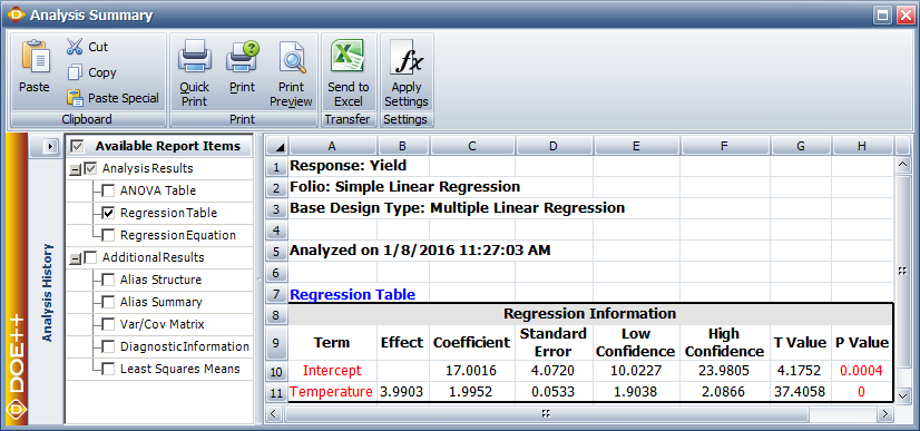
Analysis of Variance Approach to Test the Significance of Regression
The analysis of variance (ANOVA) is another method to test for the significance of regression. As the name implies, this approach uses the variance of the observed data to determine if a regression model can be applied to the observed data. The observed variance is partitioned into components that are then used in the test for significance of regression.
Sum of Squares
The total variance (i.e., the variance of all of the observed data) is estimated using the observed data. As mentioned in Statistical Background, the variance of a population can be estimated using the sample variance, which is calculated using the following relationship:
- [math]\displaystyle{ {{s}^{2}}=\frac{\underset{i=1}{\overset{n}{\mathop{\sum }}}\,{{({{y}_{i}}-\bar{y})}^{2}}}{n-1}\,\! }[/math]
The quantity in the numerator of the previous equation is called the sum of squares. It is the sum of the square of deviations of all the observations, [math]\displaystyle{ {{y}_{i}}\,\! }[/math], from their mean, [math]\displaystyle{ \bar{y}\,\! }[/math]. In the context of ANOVA this quantity is called the total sum of squares (abbreviated [math]\displaystyle{ S{{S}_{T}}\,\! }[/math]) because it relates to the total variance of the observations. Thus:
- [math]\displaystyle{ S{{S}_{T}}=\underset{i=1}{\overset{n}{\mathop \sum }}\,{{({{y}_{i}}-\bar{y})}^{2}}\,\! }[/math]
The denominator in the relationship of the sample variance is the number of degrees of freedom associated with the sample variance. Therefore, the number of degrees of freedom associated with [math]\displaystyle{ S{{S}_{T}}\,\! }[/math], [math]\displaystyle{ dof(S{{S}_{T}})\,\! }[/math], is [math]\displaystyle{ n-1\,\! }[/math]. The sample variance is also referred to as a mean square because it is obtained by dividing the sum of squares by the respective degrees of freedom. Therefore, the total mean square (abbreviated [math]\displaystyle{ M{{S}_{T}}\,\! }[/math]) is:
- [math]\displaystyle{ M{{S}_{T}}=\frac{S{{S}_{T}}}{dof(S{{S}_{T}})}=\frac{S{{S}_{T}}}{n-1}\,\! }[/math]
When you attempt to fit a regression model to the observations, you are trying to explain some of the variation of the observations using this model. If the regression model is such that the resulting fitted regression line passes through all of the observations, then you would have a "perfect" model (see (a) of the figure below). In this case the model would explain all of the variability of the observations. Therefore, the model sum of squares (also referred to as the regression sum of squares and abbreviated [math]\displaystyle{ S{{S}_{R}}\,\! }[/math]) equals the total sum of squares; i.e., the model explains all of the observed variance:
- [math]\displaystyle{ S{{S}_{R}}=S{{S}_{T}}\,\! }[/math]
For the perfect model, the regression sum of squares, [math]\displaystyle{ S{{S}_{R}}\,\! }[/math], equals the total sum of squares, [math]\displaystyle{ S{{S}_{T}}\,\! }[/math], because all estimated values, [math]\displaystyle{ {{\hat{y}}_{i}}\,\! }[/math], will equal the corresponding observations, [math]\displaystyle{ {{y}_{i}}\,\! }[/math]. [math]\displaystyle{ S{{S}_{R}}\,\! }[/math] can be calculated using a relationship similar to the one for obtaining [math]\displaystyle{ S{{S}_{T}}\,\! }[/math] by replacing [math]\displaystyle{ {{y}_{i}}\,\! }[/math] by [math]\displaystyle{ {{\hat{y}}_{i}}\,\! }[/math] in the relationship of [math]\displaystyle{ S{{S}_{T}}\,\! }[/math]. Therefore:
- [math]\displaystyle{ S{{S}_{R}}=\underset{i=1}{\overset{n}{\mathop \sum }}\,{{({{\hat{y}}_{i}}-\bar{y})}^{2}}\,\! }[/math]
The number of degrees of freedom associated with [math]\displaystyle{ S{{S}_{R}}\,\! }[/math] is 1.
Based on the preceding discussion of ANOVA, a perfect regression model exists when the fitted regression line passes through all observed points. However, this is not usually the case, as seen in (b) of the following figure.
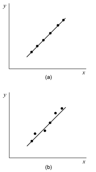
In both of these plots, a number of points do not follow the fitted regression line. This indicates that a part of the total variability of the observed data still remains unexplained. This portion of the total variability or the total sum of squares, that is not explained by the model, is called the residual sum of squares or the error sum of squares (abbreviated [math]\displaystyle{ S{{S}_{E}}\,\! }[/math]). The deviation for this sum of squares is obtained at each observation in the form of the residuals, [math]\displaystyle{ {{e}_{i}}\,\! }[/math]. The error sum of squares can be obtained as the sum of squares of these deviations:
- [math]\displaystyle{ S{{S}_{E}}=\underset{i=1}{\overset{n}{\mathop \sum }}\,e_{i}^{2}=\underset{i=1}{\overset{n}{\mathop \sum }}\,{{({{y}_{i}}-{{\hat{y}}_{i}})}^{2}}\,\! }[/math]
The number of degrees of freedom associated with [math]\displaystyle{ S{{S}_{E}}\,\! }[/math], [math]\displaystyle{ dof(S{{S}_{E}})\,\! }[/math], is [math]\displaystyle{ (n-2)\,\! }[/math].
The total variability of the observed data (i.e., total sum of squares, [math]\displaystyle{ S{{S}_{T}}\,\! }[/math]) can be written using the portion of the variability explained by the model, [math]\displaystyle{ S{{S}_{R}}\,\! }[/math], and the portion unexplained by the model, [math]\displaystyle{ S{{S}_{E}}\,\! }[/math], as:
- [math]\displaystyle{ S{{S}_{T}}=S{{S}_{R}}+S{{S}_{E}}\,\! }[/math]
The above equation is also referred to as the analysis of variance identity and can be expanded as follows:
- [math]\displaystyle{ \underset{i=1}{\overset{n}{\mathop \sum }}\,{{({{y}_{i}}-\bar{y})}^{2}}=\underset{i=1}{\overset{n}{\mathop \sum }}\,{{({{\hat{y}}_{i}}-\bar{y})}^{2}}+\underset{i=1}{\overset{n}{\mathop \sum }}\,{{({{y}_{i}}-{{\hat{y}}_{i}})}^{2}}\,\! }[/math]
![Scatter plots showing the deviations for the sum of squares used in ANOVA. (a) shows deviations for [math]\displaystyle{ S S_{T}\,\! }[/math], (b) shows deviations for [math]\displaystyle{ S S_{R}\,\! }[/math], and (c) shows deviations for [math]\displaystyle{ S S_{E}\,\! }[/math]. Scatter plots showing the deviations for the sum of squares used in ANOVA. (a) shows deviations for [math]\displaystyle{ S S_{T}\,\! }[/math], (b) shows deviations for [math]\displaystyle{ S S_{R}\,\! }[/math], and (c) shows deviations for [math]\displaystyle{ S S_{E}\,\! }[/math].](/images/thumb/8/81/Doe4.9.png/600px-Doe4.9.png)
Mean Squares
As mentioned previously, mean squares are obtained by dividing the sum of squares by the respective degrees of freedom. For example, the error mean square, [math]\displaystyle{ M{{S}_{E}}\,\! }[/math], can be obtained as:
- [math]\displaystyle{ M{{S}_{E}}=\frac{S{{S}_{E}}}{dof(S{{S}_{E}})}=\frac{S{{S}_{E}}}{n-2}\,\! }[/math]
The error mean square is an estimate of the variance, [math]\displaystyle{ {{\sigma }^{2}}\,\! }[/math], of the random error term, [math]\displaystyle{ \epsilon\,\! }[/math], and can be written as:
- [math]\displaystyle{ {{\hat{\sigma }}^{2}}=\frac{S{{S}_{E}}}{n-2}\,\! }[/math]
Similarly, the regression mean square, [math]\displaystyle{ M{{S}_{R}}\,\! }[/math], can be obtained by dividing the regression sum of squares by the respective degrees of freedom as follows:
- [math]\displaystyle{ M{{S}_{R}}=\frac{S{{S}_{R}}}{dof(S{{S}_{R}})}=\frac{S{{S}_{R}}}{1}\,\! }[/math]
F Test
To test the hypothesis [math]\displaystyle{ {{H}_{0}}:{{\beta }_{1}}=0\,\! }[/math], the statistic used is based on the [math]\displaystyle{ F\,\! }[/math] distribution. It can be shown that if the null hypothesis [math]\displaystyle{ {{H}_{0}}\,\! }[/math] is true, then the statistic:
- [math]\displaystyle{ {{F}_{0}}=\frac{M{{S}_{R}}}{M{{S}_{E}}}=\frac{S{{S}_{R}}/1}{S{{S}_{E}}/(n-2)}\,\! }[/math]
follows the [math]\displaystyle{ F\,\! }[/math] distribution with [math]\displaystyle{ 1\,\! }[/math] degree of freedom in the numerator and [math]\displaystyle{ (n-2)\,\! }[/math] degrees of freedom in the denominator. [math]\displaystyle{ {{H}_{0}}\,\! }[/math] is rejected if the calculated statistic, [math]\displaystyle{ {{F}_{0}}\,\! }[/math], is such that:
- [math]\displaystyle{ {{F}_{0}}\gt {{f}_{\alpha ,1,n-2}}\,\! }[/math]
where [math]\displaystyle{ {{f}_{\alpha ,1,n-2}}\,\! }[/math] is the percentile of the [math]\displaystyle{ F\,\! }[/math] distribution corresponding to a cumulative probability of ([math]\displaystyle{ 1-\alpha\,\! }[/math]) and [math]\displaystyle{ \alpha\,\! }[/math] is the significance level.
Example
The analysis of variance approach to test the significance of regression can be applied to the yield data in the preceding table. To calculate the statistic, [math]\displaystyle{ {{F}_{0}}\,\! }[/math], for the test, the sum of squares have to be obtained. The sum of squares can be calculated as shown next. The total sum of squares can be calculated as:
- [math]\displaystyle{ \begin{align} S{{S}_{T}}= & \underset{i=1}{\overset{n}{\mathop \sum }}\,{{({{y}_{i}}-\bar{y})}^{2}} \\ = & \underset{i=1}{\overset{25}{\mathop \sum }}\,{{({{y}_{i}}-166.32)}^{2}} \\ = & 22979.44 \end{align}\,\! }[/math]
The regression sum of squares can be calculated as:
- [math]\displaystyle{ \begin{align} S{{S}_{R}}= & \underset{i=1}{\overset{n}{\mathop \sum }}\,{{({{{\hat{y}}}_{i}}-\bar{y})}^{2}} \\ = & \underset{i=1}{\overset{25}{\mathop \sum }}\,{{({{{\hat{y}}}_{i}}-166.32)}^{2}} \\ = & 22607.81 \end{align}\,\! }[/math]
The error sum of squares can be calculated as:
- [math]\displaystyle{ \begin{align} S{{S}_{E}}= & \underset{i=1}{\overset{n}{\mathop \sum }}\,{{({{y}_{i}}-{{{\hat{y}}}_{i}})}^{2}} \\ = & \underset{i=1}{\overset{25}{\mathop \sum }}\,{{({{y}_{i}}-{{{\hat{y}}}_{i}})}^{2}} \\ = & 371.63 \end{align}\,\! }[/math]
Knowing the sum of squares, the statistic to test [math]\displaystyle{ {{H}_{0}}:{{\beta }_{1}}=0\,\! }[/math] can be calculated as follows:
- [math]\displaystyle{ \begin{align} {{f}_{0}}=& \frac{M{{S}_{R}}}{M{{S}_{E}}} \\ = & \frac{S{{S}_{R}}/1}{S{{S}_{E}}/(n-2)} \\ = & \frac{22607.81/1}{371.63/(25-2)} \\ = & 1399.20 \end{align}\,\! }[/math]
The critical value at a significance level of 0.1 is [math]\displaystyle{ {{f}_{0.05,1,23}}=2.937\,\! }[/math]. Since [math]\displaystyle{ {{f}_{0}}\gt {{f}_{\alpha ,1,n-2}}\,\! }[/math], [math]\displaystyle{ {{H}_{0}}:{{\beta }_{1}}=0\,\! }[/math] is rejected and it is concluded that [math]\displaystyle{ {{\beta }_{1}}\,\! }[/math] is not zero. Alternatively, the [math]\displaystyle{ p\,\! }[/math] value can also be used. The [math]\displaystyle{ p\,\! }[/math] value corresponding to the test statistic, [math]\displaystyle{ {{f}_{0}}\,\! }[/math], based on the [math]\displaystyle{ F\,\! }[/math] distribution with one degree of freedom in the numerator and 23 degrees of freedom in the denominator is:
- [math]\displaystyle{ \begin{align} p\text{ }value= & 1-P(F\le {{f}_{0}}) \\ = & 1-0.999999 \\ = & 4.17E-22 \end{align}\,\! }[/math]
Assuming that the desired significance is 0.1, since the [math]\displaystyle{ p\,\! }[/math] value < 0.1, then [math]\displaystyle{ {{H}_{0}}:{{\beta }_{1}}=0\,\! }[/math] is rejected, implying that a relation does exist between temperature and yield for the data in the preceding table. Using this result along with the scatter plot of the above figure, it can be concluded that the relationship that exists between temperature and yield is linear. This result is displayed in the ANOVA table as shown in the following figure. Note that this is the same result that was obtained from the [math]\displaystyle{ t\,\! }[/math] test in the section t Tests. The ANOVA and Regression Information tables in Weibull++ DOE folios represent two different ways to test for the significance of the regression model. In the case of multiple linear regression models these tables are expanded to allow tests on individual variables used in the model. This is done using extra sum of squares. Multiple linear regression models and the application of extra sum of squares in the analysis of these models are discussed in Multiple Linear Regression Analysis.
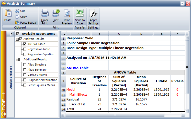
Confidence Intervals in Simple Linear Regression
A confidence interval represents a closed interval where a certain percentage of the population is likely to lie. For example, a 90% confidence interval with a lower limit of [math]\displaystyle{ A\,\! }[/math] and an upper limit of [math]\displaystyle{ B\,\! }[/math] implies that 90% of the population lies between the values of [math]\displaystyle{ A\,\! }[/math] and [math]\displaystyle{ B\,\! }[/math]. Out of the remaining 10% of the population, 5% is less than [math]\displaystyle{ A\,\! }[/math] and 5% is greater than [math]\displaystyle{ B\,\! }[/math]. (For details refer to the Life data analysis reference.) This section discusses confidence intervals used in simple linear regression analysis.
Confidence Interval on Regression Coefficients
A 100 ([math]\displaystyle{ 1-\alpha\,\! }[/math]) percent confidence interval on [math]\displaystyle{ {{\beta }_{1}}\,\! }[/math] is obtained as follows:
- [math]\displaystyle{ {{\hat{\beta }}_{1}}\pm {{t}_{\alpha /2,n-2}}\cdot se({{\hat{\beta }}_{1}})\,\! }[/math]
Similarly, a 100 ([math]\displaystyle{ 1-\alpha\,\! }[/math]) percent confidence interval on [math]\displaystyle{ {{\beta }_{0}}\,\! }[/math] is obtained as:
- [math]\displaystyle{ {{\hat{\beta }}_{0}}\pm {{t}_{\alpha /2,n-2}}\cdot se({{\hat{\beta }}_{0}})\,\! }[/math]
Confidence Interval on Fitted Values
A 100 ([math]\displaystyle{ 1-\alpha\,\! }[/math]) percent confidence interval on any fitted value, [math]\displaystyle{ {{\hat{y}}_{i}}\,\! }[/math], is obtained as follows:
- [math]\displaystyle{ {{\hat{y}}_{i}}\pm {{t}_{\alpha /2,n-2}}\sqrt{{{{\hat{\sigma }}}^{2}}\left[ \frac{1}{n}+\frac{{{({{x}_{i}}-\bar{x})}^{2}}}{\underset{i=1}{\overset{n}{\mathop \sum }}\,{{({{x}_{i}}-\bar{x})}^{2}}} \right]}\,\! }[/math]
It can be seen that the width of the confidence interval depends on the value of [math]\displaystyle{ {{x}_{i}}\,\! }[/math] and will be a minimum at [math]\displaystyle{ {{x}_{i}}=\bar{x}\,\! }[/math] and will widen as [math]\displaystyle{ \left| {{x}_{i}}-\bar{x} \right|\,\! }[/math] increases.
Confidence Interval on New Observations
For the data in the preceding table, assume that a new value of the yield is observed after the regression model is fit to the data. This new observation is independent of the observations used to obtain the regression model. If [math]\displaystyle{ {{x}_{p}}\,\! }[/math] is the level of the temperature at which the new observation was taken, then the estimate for this new value based on the fitted regression model is:
- [math]\displaystyle{ \begin{align} {{{\hat{y}}}_{p}}= & {{{\hat{\beta }}}_{0}}+{{{\hat{\beta }}}_{1}}{{x}_{p}} \\ = & 17.0016+1.9952\times {{x}_{p}} \\ \end{align}\,\! }[/math]
If a confidence interval needs to be obtained on [math]\displaystyle{ {{\hat{y}}_{p}}\,\! }[/math], then this interval should include both the error from the fitted model and the error associated with future observations. This is because [math]\displaystyle{ {{\hat{y}}_{p}}\,\! }[/math] represents the estimate for a value of [math]\displaystyle{ Y\,\! }[/math] that was not used to obtain the regression model. The confidence interval on [math]\displaystyle{ {{\hat{y}}_{p}}\,\! }[/math] is referred to as the prediction interval. A 100 ([math]\displaystyle{ 1-\alpha\,\! }[/math]) percent prediction interval on a new observation is obtained as follows:
- [math]\displaystyle{ {{\hat{y}}_{p}}\pm {{t}_{\alpha /2,n-2}}\sqrt{{{{\hat{\sigma }}}^{2}}\left[ 1+\frac{1}{n}+\frac{{{({{x}_{p}}-\bar{x})}^{2}}}{\underset{i=1}{\overset{n}{\mathop \sum }}\,{{({{x}_{p}}-\bar{x})}^{2}}} \right]}\,\! }[/math]
Example
To illustrate the calculation of confidence intervals, the 95% confidence intervals on the response at [math]\displaystyle{ x=93\,\! }[/math] for the data in the preceding table is obtained in this example. A 95% prediction interval is also obtained assuming that a new observation for the yield was made at [math]\displaystyle{ x=91\,\! }[/math].
The fitted value, [math]\displaystyle{ {{\hat{y}}_{i}}\,\! }[/math], corresponding to [math]\displaystyle{ x=93\,\! }[/math] is:
- [math]\displaystyle{ \begin{align} {{{\hat{y}}}_{21}}= & {{{\hat{\beta }}}_{0}}+{{{\hat{\beta }}}_{1}}{{x}_{21}} \\ = & 17.0016+1.9952\times 93 \\ = & 202.6 \end{align}\,\! }[/math]
The 95% confidence interval [math]\displaystyle{ (\alpha =0.05)\,\! }[/math] on the fitted value, [math]\displaystyle{ {{\hat{y}}_{21}}=202.6\,\! }[/math], is:
- [math]\displaystyle{ \begin{align} = & {{{\hat{y}}}_{i}}\pm {{t}_{\alpha /2,n-2}}\sqrt{{{{\hat{\sigma }}}^{2}}\left[ \frac{1}{n}+\frac{{{({{x}_{i}}-\bar{x})}^{2}}}{\underset{i=1}{\overset{n}{\mathop \sum }}\,{{({{x}_{i}}-\bar{x})}^{2}}} \right]} \\ = & 202.6\pm {{t}_{0.025,23}}\sqrt{M{{S}_{E}}\left[ \frac{1}{25}+\frac{{{(93-74.84)}^{2}}}{5679.36} \right]} \\ = & 202.6\pm 2.069\sqrt{16.16\left[ \frac{1}{25}+\frac{{{(93-74.84)}^{2}}}{5679.36} \right]} \\ = & 202.6\pm 2.602 \end{align}\,\! }[/math]
The 95% limits on [math]\displaystyle{ {{\hat{y}}_{21}}\,\! }[/math] are 199.95 and 205.2, respectively.
The estimated value based on the fitted regression model for the new observation at [math]\displaystyle{ x=91\,\! }[/math] is:
- [math]\displaystyle{ \begin{align} {{{\hat{y}}}_{p}}= & {{{\hat{\beta }}}_{0}}+{{{\hat{\beta }}}_{1}}{{x}_{p}} \\ = & 17.0016+1.9952\times 91 \\ = & 198.6 \end{align}\,\! }[/math]
The 95% prediction interval on [math]\displaystyle{ {{\hat{y}}_{p}}=198.6\,\! }[/math] is:
- [math]\displaystyle{ \begin{align} = & {{{\hat{y}}}_{p}}\pm {{t}_{\alpha /2,n-2}}\sqrt{{{{\hat{\sigma }}}^{2}}\left[ 1+\frac{1}{n}+\frac{{{({{x}_{p}}-\bar{x})}^{2}}}{\underset{i=1}{\overset{n}{\mathop \sum }}\,{{({{x}_{p}}-\bar{x})}^{2}}} \right]} \\ = & 198.6\pm {{t}_{0.025,23}}\sqrt{M{{S}_{E}}\left[ 1+\frac{1}{25}+\frac{{{(93-74.84)}^{2}}}{5679.36} \right]} \\ = & 198.6\pm 2.069\sqrt{16.16\left[ 1+\frac{1}{25}+\frac{{{(93-74.84)}^{2}}}{5679.36} \right]} \\ = & 198.6\pm 2.069\times 4.1889 \\ = & 198.6\pm 8.67 \end{align}\,\! }[/math]
The 95% limits on [math]\displaystyle{ {{\hat{y}}_{p}}\,\! }[/math] are 189.9 and 207.2, respectively. In Weibull++ DOE folios, confidence and prediction intervals can be calculated from the control panel. The prediction interval values calculated in this example are shown in the figure below as Low Prediction Interval and High Prediction Interval, respectively. The columns labeled Mean Predicted and Standard Error represent the values of [math]\displaystyle{ {{\hat{y}}_{p}}\,\! }[/math] and the standard error used in the calculations.
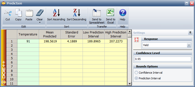
Measures of Model Adequacy
It is important to analyze the regression model before inferences based on the model are undertaken. The following sections present some techniques that can be used to check the appropriateness of the model for the given data. These techniques help to determine if any of the model assumptions have been violated.
Coefficient of Determination ([math]\displaystyle{ R^2 }[/math])
The coefficient of determination is a measure of the amount of variability in the data accounted for by the regression model. As mentioned previously, the total variability of the data is measured by the total sum of squares, [math]\displaystyle{ SS_T\,\! }[/math]. The amount of this variability explained by the regression model is the regression sum of squares, [math]\displaystyle{ SS_R\,\! }[/math]. The coefficient of determination is the ratio of the regression sum of squares to the total sum of squares.
- [math]\displaystyle{ R^2 = \frac{SS_R}{SS_T}\,\! }[/math]
[math]\displaystyle{ R^2\,\! }[/math] can take on values between 0 and 1 since [math]\displaystyle{ R^2 = \frac{SS_R}{SS_T}\,\! }[/math] . For the yield data example, [math]\displaystyle{ R^2\,\! }[/math] can be calculated as:
- [math]\displaystyle{ \begin{align} {{R}^{2}}= & \frac{S{{S}_{R}}}{S{{S}_{T}}} \\ = & \frac{22607.81}{22979.44} \\ = & 0.98 \end{align}\,\! }[/math]
Therefore, 98% of the variability in the yield data is explained by the regression model, indicating a very good fit of the model. It may appear that larger values of [math]\displaystyle{ {{R}^{2}}\,\! }[/math] indicate a better fitting regression model. However, [math]\displaystyle{ {{R}^{2}}\,\! }[/math] should be used cautiously as this is not always the case. The value of [math]\displaystyle{ {{R}^{2}}\,\! }[/math] increases as more terms are added to the model, even if the new term does not contribute significantly to the model. Therefore, an increase in the value of [math]\displaystyle{ {{R}^{2}}\,\! }[/math] cannot be taken as a sign to conclude that the new model is superior to the older model. Adding a new term may make the regression model worse if the error mean square, [math]\displaystyle{ M{{S}_{E}}\,\! }[/math], for the new model is larger than the [math]\displaystyle{ M{{S}_{E}}\,\! }[/math] of the older model, even though the new model will show an increased value of [math]\displaystyle{ {{R}^{2}}\,\! }[/math]. In the results obtained from the DOE folio, [math]\displaystyle{ {{R}^{2}}\,\! }[/math] is displayed as R-sq under the ANOVA table (as shown in the figure below), which displays the complete analysis sheet for the data in the preceding table.
The other values displayed with are S, R-sq(adj), PRESS and R-sq(pred). These values measure different aspects of the adequacy of the regression model. For example, the value of S is the square root of the error mean square, [math]\displaystyle{ MS_E\,\! }[/math], and represents the "standard error of the model." A lower value of S indicates a better fitting model. The values of S, R-sq and R-sq(adj) indicate how well the model fits the observed data. The values of PRESS and R-sq(pred) are indicators of how well the regression model predicts new observations. R-sq(adj), PRESS and R-sq(pred) are explained in Multiple Linear Regression Analysis.
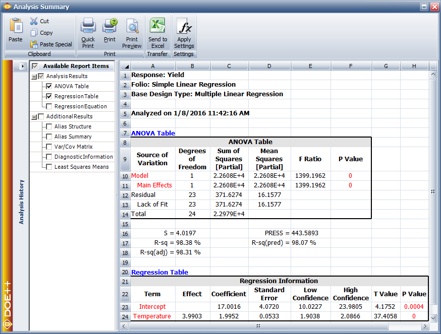
Residual Analysis
In the simple linear regression model the true error terms, [math]\displaystyle{ {{\epsilon }_{i}}\,\! }[/math], are never known. The residuals, [math]\displaystyle{ {{e}_{i}}\,\! }[/math], may be thought of as the observed error terms that are similar to the true error terms. Since the true error terms, [math]\displaystyle{ {{\epsilon }_{i}}\,\! }[/math], are assumed to be normally distributed with a mean of zero and a variance of [math]\displaystyle{ {{\sigma }^{2}}\,\! }[/math], in a good model the observed error terms (i.e., the residuals, [math]\displaystyle{ {{e}_{i}}\,\! }[/math]) should also follow these assumptions. Thus the residuals in the simple linear regression should be normally distributed with a mean of zero and a constant variance of [math]\displaystyle{ {{\sigma }^{2}}\,\! }[/math]. Residuals are usually plotted against the fitted values, [math]\displaystyle{ {{\hat{y}}_{i}}\,\! }[/math], against the predictor variable values, [math]\displaystyle{ {{x}_{i}}\,\! }[/math], and against time or run-order sequence, in addition to the normal probability plot. Plots of residuals are used to check for the following:
- 1. Residuals follow the normal distribution.
- 2. Residuals have a constant variance.
- 3. Regression function is linear.
- 4. A pattern does not exist when residuals are plotted in a time or run-order sequence.
- 5. There are no outliers.
Examples of residual plots are shown in the following figure. (a) is a satisfactory plot with the residuals falling in a horizontal band with no systematic pattern. Such a plot indicates an appropriate regression model. (b) shows residuals falling in a funnel shape. Such a plot indicates increase in variance of residuals and the assumption of constant variance is violated here. Transformation on [math]\displaystyle{ Y\,\! }[/math] may be helpful in this case (see Transformations). If the residuals follow the pattern of (c) or (d), then this is an indication that the linear regression model is not adequate. Addition of higher order terms to the regression model or transformation on [math]\displaystyle{ x\,\! }[/math] or [math]\displaystyle{ Y\,\! }[/math] may be required in such cases. A plot of residuals may also show a pattern as seen in (e), indicating that the residuals increase (or decrease) as the run order sequence or time progresses. This may be due to factors such as operator-learning or instrument-creep and should be investigated further.
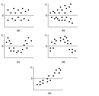
Example
Residual plots for the data of the preceding table are shown in the following figures. One of the following figures is the normal probability plot. It can be observed that the residuals follow the normal distribution and the assumption of normality is valid here. In one of the following figures the residuals are plotted against the fitted values, [math]\displaystyle{ {{\hat{y}}_{i}}\,\! }[/math], and in one of the following figures the residuals are plotted against the run order. Both of these plots show that the 21st observation seems to be an outlier. Further investigations are needed to study the cause of this outlier.
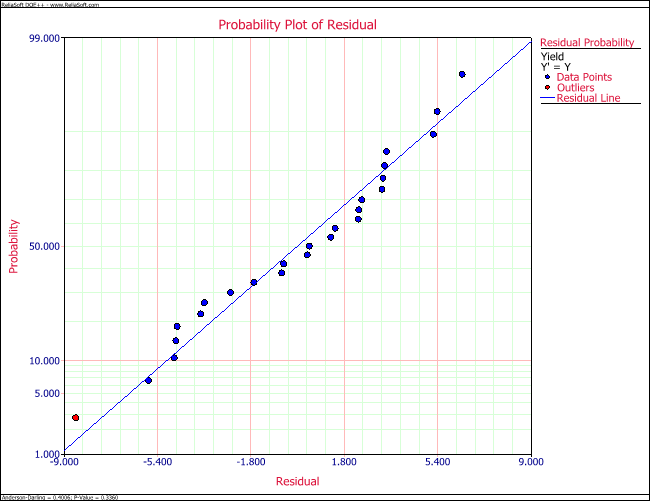
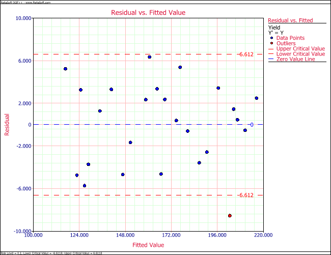
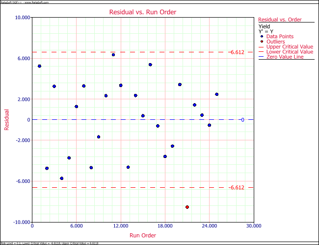
Lack-of-Fit Test
As mentioned in Analysis of Variance Approach, ANOVA, a perfect regression model results in a fitted line that passes exactly through all observed data points. This perfect model will give us a zero error sum of squares ([math]\displaystyle{ S{{S}_{E}}=0\,\! }[/math]). Thus, no error exists for the perfect model. However, if you record the response values for the same values of [math]\displaystyle{ {{x}_{i}}\,\! }[/math] for a second time, in conditions maintained as strictly identical as possible to the first time, observations from the second time will not all fall along the perfect model. The deviations in observations recorded for the second time constitute the "purely" random variation or noise. The sum of squares due to pure error (abbreviated [math]\displaystyle{ S{{S}_{PE}}\,\! }[/math]) quantifies these variations. [math]\displaystyle{ S{{S}_{PE}}\,\! }[/math] is calculated by taking repeated observations at some or all values of [math]\displaystyle{ {{x}_{i}}\,\! }[/math] and adding up the square of deviations at each level of [math]\displaystyle{ x\,\! }[/math] using the respective repeated observations at that [math]\displaystyle{ x\,\! }[/math] value.
Assume that there are [math]\displaystyle{ n\,\! }[/math] levels of [math]\displaystyle{ x\,\! }[/math] and [math]\displaystyle{ {{m}_{i}}\,\! }[/math] repeated observations are taken at each [math]\displaystyle{ i\,\! }[/math] the level. The data is collected as shown next:
- [math]\displaystyle{ \begin{align} & {{y}_{11}},{{y}_{12}},....,{{y}_{1{{m}_{1}}}}\text{ repeated observations at }{{x}_{1}} \\ & {{y}_{21}},{{y}_{22}},....,{{y}_{2{{m}_{2}}}}\text{ repeated observations at }{{x}_{2}} \\ & ... \\ & {{y}_{i1}},{{y}_{i2}},....,{{y}_{i{{m}_{i}}}}\text{ repeated observations at }{{x}_{i}} \\ & ... \\ & {{y}_{n1}},{{y}_{n2}},....,{{y}_{n{{m}_{n}}}}\text{ repeated observations at }{{x}_{n}} \end{align}\,\! }[/math]
The sum of squares of the deviations from the mean of the observations at [math]\displaystyle{ i\,\! }[/math] the level of [math]\displaystyle{ x\,\! }[/math], [math]\displaystyle{ {{x}_{i}}\,\! }[/math], can be calculated as:
- [math]\displaystyle{ \underset{j=1}{\overset{{{m}_{i}}}{\mathop \sum }}\,{{({{y}_{ij}}-{{\bar{y}}_{i}})}^{2}}\,\! }[/math]
where [math]\displaystyle{ {{\bar{y}}_{i}}\,\! }[/math] is the mean of the [math]\displaystyle{ {{m}_{i}}\,\! }[/math] repeated observations corresponding to [math]\displaystyle{ {{x}_{i}}\,\! }[/math] ([math]\displaystyle{ {{\bar{y}}_{i}}=(1/{{m}_{i}})\mathop{}_{j=1}^{{{m}_{i}}}{{y}_{ij}}\,\! }[/math]). The number of degrees of freedom for these deviations is ([math]\displaystyle{ {{m}_{i}}-1\,\! }[/math] ) as there are [math]\displaystyle{ {{m}_{i}}\,\! }[/math] observations at [math]\displaystyle{ i\,\! }[/math] the level of [math]\displaystyle{ x\,\! }[/math] but one degree of freedom is lost in calculating the mean, [math]\displaystyle{ {{\bar{y}}_{i}}\,\! }[/math].
The total sum of square deviations (or [math]\displaystyle{ S{{S}_{PE}}\,\! }[/math]) for all levels of [math]\displaystyle{ x\,\! }[/math] can be obtained by summing the deviations for all [math]\displaystyle{ {{x}_{i}}\,\! }[/math] as shown next:
- [math]\displaystyle{ S{{S}_{PE}}=\underset{i=1}{\overset{n}{\mathop \sum }}\,\underset{j=1}{\overset{{{m}_{i}}}{\mathop \sum }}\,{{({{y}_{ij}}-{{\bar{y}}_{i}})}^{2}}\,\! }[/math]
The total number of degrees of freedom associated with [math]\displaystyle{ S{{S}_{PE}}\,\! }[/math] is:
- [math]\displaystyle{ \begin{align} = & \underset{i=1}{\overset{n}{\mathop \sum }}\,({{m}_{i}}-1) \\ = & \underset{i=1}{\overset{n}{\mathop \sum }}\,{{m}_{i}}-n \end{align}\,\! }[/math]
If all [math]\displaystyle{ {{m}_{i}}=m\,\! }[/math], (i.e., [math]\displaystyle{ m\,\! }[/math] repeated observations are taken at all levels of [math]\displaystyle{ x\,\! }[/math]), then [math]\displaystyle{ \mathop{}_{i=1}^{n}{{m}_{i}}=nm\,\! }[/math] and the degrees of freedom associated with [math]\displaystyle{ S{{S}_{PE}}\,\! }[/math] are:
- [math]\displaystyle{ =nm-n\,\! }[/math]
The corresponding mean square in this case will be:
- [math]\displaystyle{ M{{S}_{PE}}=\frac{S{{S}_{PE}}}{nm-n}\,\! }[/math]
When repeated observations are used for a perfect regression model, the sum of squares due to pure error, [math]\displaystyle{ S{{S}_{PE}}\,\! }[/math], is also considered as the error sum of squares, [math]\displaystyle{ S{{S}_{E}}\,\! }[/math]. For the case when repeated observations are used with imperfect regression models, there are two components of the error sum of squares, [math]\displaystyle{ S{{S}_{E}}\,\! }[/math]. One portion is the pure error due to the repeated observations. The other portion is the error that represents variation not captured because of the imperfect model. The second portion is termed as the sum of squares due to lack-of-fit (abbreviated [math]\displaystyle{ S{{S}_{LOF}}\,\! }[/math]) to point to the deficiency in fit due to departure from the perfect-fit model. Thus, for an imperfect regression model:
- [math]\displaystyle{ S{{S}_{E}}=S{{S}_{PE}}+S{{S}_{LOF}}\,\! }[/math]
Knowing [math]\displaystyle{ S{{S}_{E}}\,\! }[/math] and [math]\displaystyle{ S{{S}_{PE}}\,\! }[/math], the previous equation can be used to obtain [math]\displaystyle{ S{{S}_{LOF}}\,\! }[/math]:
- [math]\displaystyle{ S{{S}_{LOF}}=S{{S}_{E}}-S{{S}_{PE}}\,\! }[/math]
The degrees of freedom associated with [math]\displaystyle{ S{{S}_{LOF}}\,\! }[/math] can be obtained in a similar manner using subtraction. For the case when [math]\displaystyle{ m\,\! }[/math] repeated observations are taken at all levels of [math]\displaystyle{ x\,\! }[/math], the number of degrees of freedom associated with [math]\displaystyle{ S{{S}_{PE}}\,\! }[/math] is:
- [math]\displaystyle{ dof(S{{S}_{PE}})=nm-n\,\! }[/math]
Since there are [math]\displaystyle{ nm\,\! }[/math] total observations, the number of degrees of freedom associated with [math]\displaystyle{ S{{S}_{E}}\,\! }[/math] is:
- [math]\displaystyle{ dof(S{{S}_{E}})=nm-2\,\! }[/math]
Therefore, the number of degrees of freedom associated with [math]\displaystyle{ S{{S}_{LOF}}\,\! }[/math] is:
- [math]\displaystyle{ \begin{align} = & dof(S{{S}_{E}})-dof(S{{S}_{PE}}) \\ = & (nm-2)-(nm-n) \\ = & n-2 \end{align}\,\! }[/math]
The corresponding mean square, [math]\displaystyle{ M{{S}_{LOF}}\,\! }[/math], can now be obtained as:
- [math]\displaystyle{ M{{S}_{LOF}}=\frac{S{{S}_{LOF}}}{n-2}\,\! }[/math]
The magnitude of [math]\displaystyle{ S{{S}_{LOF}}\,\! }[/math] or [math]\displaystyle{ M{{S}_{LOF}}\,\! }[/math] will provide an indication of how far the regression model is from the perfect model. An [math]\displaystyle{ F\,\! }[/math] test exists to examine the lack-of-fit at a particular significance level. The quantity [math]\displaystyle{ M{{S}_{LOF}}/M{{S}_{PE}}\,\! }[/math] follows an [math]\displaystyle{ F\,\! }[/math] distribution with [math]\displaystyle{ (n-2)\,\! }[/math] degrees of freedom in the numerator and [math]\displaystyle{ (nm-n)\,\! }[/math] degrees of freedom in the denominator when all [math]\displaystyle{ {{m}_{i}}\,\! }[/math] equal [math]\displaystyle{ m\,\! }[/math]. The test statistic for the lack-of-fit test is:
- [math]\displaystyle{ {{F}_{0}}=\frac{M{{S}_{LOF}}}{M{{S}_{PE}}}\,\! }[/math]
If the critical value [math]\displaystyle{ {{f}_{\alpha ,n-2,mn-n}}\,\! }[/math] is such that:
- [math]\displaystyle{ {{F}_{0}}\gt {{f}_{\alpha ,n-2,nm-n}}\,\! }[/math]
it will lead to the rejection of the hypothesis that the model adequately fits the data.
Example
Assume that a second set of observations are taken for the yield data of the preceding table. The resulting observations are recorded in the following table. To conduct a lack-of-fit test on this data, the statistic [math]\displaystyle{ {{F}_{0}}=M{{S}_{LOF}}/M{{S}_{PE}}\,\! }[/math], can be calculated as shown next.
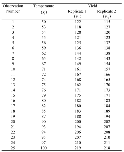
Calculation of Least Square Estimates
The parameters of the fitted regression model can be obtained as:
- [math]\displaystyle{ \begin{align} {{{\hat{\beta }}}_{1}} = & \frac{\underset{i=1}{\overset{50}{\mathop \sum }}\,{{y}_{i}}{{x}_{i}}-\frac{\left( \underset{i=1}{\overset{50}{\mathop \sum }}\,{{y}_{i}} \right)\left( \underset{i=1}{\overset{50}{\mathop \sum }}\,{{x}_{i}} \right)}{50}}{\underset{i=1}{\overset{50}{\mathop \sum }}\,{{({{x}_{i}}-\bar{x})}^{2}}} \\ = & \frac{648532-\frac{8356\times 3742}{50}}{11358.72} \\ = & 2.04 \end{align}\,\! }[/math]
- [math]\displaystyle{ \begin{align} {{{\hat{\beta }}}_{0}}= & \bar{y}-{{{\hat{\beta }}}_{1}}\bar{x} \\ = & 167.12-2.04\times 74.84 \\ = & 14.47 \end{align}\,\! }[/math]
Knowing [math]\displaystyle{ {{\hat{\beta }}_{1}}\,\! }[/math] and [math]\displaystyle{ {{\hat{\beta }}_{0}}\,\! }[/math], the fitted values, [math]\displaystyle{ {{\hat{y}}_{i}}\,\! }[/math], can be calculated.
Calculation of the Sum of Squares
Using the fitted values, the sum of squares can be obtained as follows:
- [math]\displaystyle{ \begin{align} S{{S}_{T}} = & \underset{i=1}{\overset{50}{\mathop \sum }}\,{{({{y}_{i}}-\bar{y})}^{2}} \\ = & 47907.28 \end{align}\,\! }[/math]
- [math]\displaystyle{ \begin{align} S{{S}_{R}} = & \underset{i=1}{\overset{50}{\mathop \sum }}\,{{({{{\hat{y}}}_{i}}-\bar{y})}^{2}} \\ = & 47258.91 \end{align} \,\! }[/math]
- [math]\displaystyle{ \begin{align} S{{S}_{E}} = & \underset{i=1}{\overset{50}{\mathop \sum }}\,{{({{y}_{i}}-{{{\hat{y}}}_{i}})}^{2}} \\ = & 648.37 \end{align} \,\! }[/math]
Calculation of [math]\displaystyle{ M{{S}_{LOF}}\,\! }[/math]
The error sum of squares, [math]\displaystyle{ S{{S}_{E}}\,\! }[/math], can now be split into the sum of squares due to pure error, [math]\displaystyle{ S{{S}_{PE}}\,\! }[/math], and the sum of squares due to lack-of-fit, [math]\displaystyle{ S{{S}_{LOF}}\,\! }[/math]. [math]\displaystyle{ S{{S}_{PE}}\,\! }[/math] can be calculated as follows considering that in this example [math]\displaystyle{ n=25\,\! }[/math] and [math]\displaystyle{ m=2\,\! }[/math]:
- [math]\displaystyle{ \begin{align} S{{S}_{PE}} & = \underset{i=1}{\overset{n}{\mathop \sum }}\,\underset{j=1}{\overset{{{m}_{i}}}{\mathop \sum }}\,{{({{y}_{ij}}-{{{\bar{y}}}_{i}})}^{2}} \\ & = \underset{i=1}{\overset{25}{\mathop \sum }}\,\underset{j=1}{\overset{2}{\mathop \sum }}\,{{({{y}_{ij}}-{{{\bar{y}}}_{i}})}^{2}} \\ & = 350 \end{align}\,\! }[/math]
The number of degrees of freedom associated with [math]\displaystyle{ S{{S}_{PE}}\,\! }[/math] is:
- [math]\displaystyle{ \begin{align} dof(S{{S}_{PE}}) & = nm-n \\ & = 25\times 2-25 \\ & = 25 \end{align}\,\! }[/math]
The corresponding mean square, [math]\displaystyle{ M{{S}_{PE}}\,\! }[/math], can now be obtained as:
- [math]\displaystyle{ \begin{align} M{{S}_{PE}} & = \frac{S{{S}_{PE}}}{dof(S{{S}_{PE}})} \\ & = \frac{350}{25} \\ & = 14 \end{align}\,\! }[/math]
[math]\displaystyle{ S{{S}_{LOF}}\,\! }[/math] can be obtained by subtraction from [math]\displaystyle{ S{{S}_{E}}\,\! }[/math] as:
- [math]\displaystyle{ \begin{align} S{{S}_{LOF}} & = S{{S}_{E}}-S{{S}_{PE}} \\ & = 648.37-350 \\ & = 298.37 \end{align}\,\! }[/math]
Similarly, the number of degrees of freedom associated with [math]\displaystyle{ S{{S}_{LOF}}\,\! }[/math] is:
- [math]\displaystyle{ \begin{align} dof(S{{S}_{LOF}}) & = dof(S{{S}_{E}})-dof(S{{S}_{PE}}) \\ & = (nm-2)-(nm-n) \\ & = 23 \end{align}\,\! }[/math]
The lack-of-fit mean square is:
- [math]\displaystyle{ \begin{align} M{{S}_{LOF}} & = \frac{M{{S}_{LOF}}}{dof(M{{S}_{LOF}})} \\ & = \frac{298.37}{23} \\ & = 12.97 \end{align}\,\! }[/math]
Calculation of the Test Statistic
The test statistic for the lack-of-fit test can now be calculated as:
- [math]\displaystyle{ \begin{align} {{f}_{0}} & = \frac{M{{S}_{LOF}}}{M{{S}_{PE}}} \\ & = \frac{12.97}{14} \\ & = 0.93 \end{align}\,\! }[/math]
The critical value for this test is:
- [math]\displaystyle{ {{f}_{0.05,23,25}}=1.97\,\! }[/math]
Since [math]\displaystyle{ {{f}_{0}}\lt {{f}_{0.05,23,25}}\,\! }[/math], we fail to reject the hypothesis that the model adequately fits the data. The [math]\displaystyle{ p\,\! }[/math] value for this case is:
- [math]\displaystyle{ \begin{align} p\text{ }value & = 1-P(F\le {{f}_{0}}) \\ & = 1-0.43 \\ & = 0.57 \end{align}\,\! }[/math]
Therefore, at a significance level of 0.05 we conclude that the simple linear regression model, [math]\displaystyle{ y=14.47+2.04x\,\! }[/math], is adequate for the observed data. The following table presents a summary of the ANOVA calculations for the lack-of-fit test.
Transformations
The linear regression model may not be directly applicable to certain data. Non-linearity may be detected from scatter plots or may be known through the underlying theory of the product or process or from past experience. Transformations on either the predictor variable, [math]\displaystyle{ x\,\! }[/math], or the response variable, [math]\displaystyle{ Y\,\! }[/math], may often be sufficient to make the linear regression model appropriate for the transformed data. If it is known that the data follows the logarithmic distribution, then a logarithmic transformation on [math]\displaystyle{ Y\,\! }[/math] (i.e., [math]\displaystyle{ {{Y}^{*}}=\log (Y)\,\! }[/math]) might be useful. For data following the Poisson distribution, a square root transformation ([math]\displaystyle{ {{Y}^{*}}=\sqrt{Y}\,\! }[/math]) is generally applicable.
Transformations on [math]\displaystyle{ Y\,\! }[/math] may also be applied based on the type of scatter plot obtained from the data. The following figure shows a few such examples.
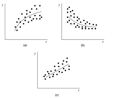
For the scatter plot labeled (a), a square root transformation ([math]\displaystyle{ {{Y}^{*}}=\sqrt{Y}\,\! }[/math]) is applicable. While for the plot labeled (b), a logarithmic transformation (i.e., [math]\displaystyle{ {{Y}^{*}}=\log (Y)\,\! }[/math]) may be applied. For the plot labeled (c), the reciprocal transformation ([math]\displaystyle{ {{Y}^{*}}=1/Y\,\! }[/math]) is applicable. At times it may be helpful to introduce a constant into the transformation of [math]\displaystyle{ Y\,\! }[/math]. For example, if [math]\displaystyle{ Y\,\! }[/math] is negative and the logarithmic transformation on [math]\displaystyle{ Y }[/math] seems applicable, a suitable constant, [math]\displaystyle{ k\,\! }[/math], may be chosen to make all observed [math]\displaystyle{ Y\,\! }[/math] positive. Thus the transformation in this case would be [math]\displaystyle{ {{Y}^{*}}=\log (k+Y)\,\! }[/math] .
The Box-Cox method may also be used to automatically identify a suitable power transformation for the data based on the relation:
- [math]\displaystyle{ {{Y}^{*}}={{Y}^{\lambda }}\,\! }[/math]
Here the parameter [math]\displaystyle{ \lambda\,\! }[/math] is determined using the given data such that [math]\displaystyle{ S{{S}_{E}}\,\! }[/math] is minimized (details on this method are presented in One Factor Designs).

