Time-Varying Stress Models

Traditionally, accelerated tests that use a time-varying stress application have been used to assure failures quickly. This is highly desirable given the pressure on industry today to shorten new product introduction time. The most basic type of time-varying stress test is a step-stress test. In step-stress accelerated testing, the test units are subjected to successively higher stress levels in predetermined stages, and thus follow a time-varying stress profile. The units usually start at a lower stress level and at a predetermined time, or failure number, the stress is increased and the test continues. The test is terminated when all units have failed, when a certain number of failures are observed or when a certain time has elapsed. Step-stress testing can substantially shorten the reliability test's duration. In addition to step-stress testing, there are many other types of time-varying stress profiles that can be used in accelerated life testing. However, it should be noted that there is more uncertainty in the results from such time-varying stress tests than from traditional constant stress tests of the same length and sample size.

When dealing with data from accelerated tests with time-varying stresses, the life-stress relationship must take into account the cumulative effect of the applied stresses. Such a model is commonly referred to as a cumulative damage or cumulative exposure model. Nelson [28] defines and presents the derivation and assumptions of such a model. ALTA includes the cumulative damage model for the analysis of time-varying stress data. This section presents an introduction to the model formulation and its application.

Model Formulation

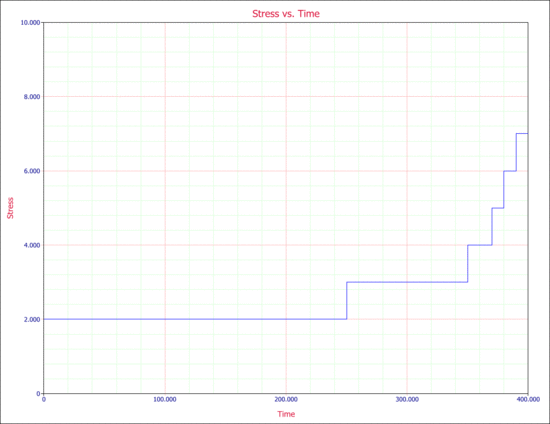
To formulate the cumulative exposure/damage model, consider a simple step-stress experiment where an electronic component was subjected to a voltage stress, starting at 2V (use stress level) and increased to 7V in stepwise increments, as shown in the next figure. The following steps, in hours, were used to apply stress to the products under test: 0 to 250, 2V; 250 to 350, 3V; 350 to 370, 4V; 370 to 380, 5V; 380 to 390, 6V; and 390 to 400, 7V.

In this example, 11 units were available for the test. All units were tested using this same stress profile. Units that failed were removed from the test and their total times on test were recorded. The following times-to-failure were observed in the test, in hours: 280, 310, 330, 352, 360, 366, 371, 374, 378, 381 and 385. The first failure in this test occurred at 280 hours when the stress was 3V. During the test, this unit experienced a period of time at 2V before failing at 3V. If the stress were 2V, one would expect the unit to fail at a time later than 280 hours, while if the unit were always at 3V, one would expect that failure time to be sooner than 280 hrs. The problem faced by the analyst in this case is to determine some equivalency between the stresses. In other words, what is the equivalent of 280 hours (with 250 hours spent at 2V and 30 hours spent at 3V) at a constant 2V stress or at a constant 3V stress?

Mathematical Formulation for a Step-Stress Model

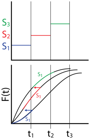
To mathematically formulate the model, consider the step-stress test shown in the next figure, with stresses S1, S2 and S3. Furthermore, assume that the underlying life distribution is the Weibull distribution, and also assume an inverse power law relationship between the Weibull scale parameter and the applied stress.

From the inverse power law relationship, the scale parameter, [math]\displaystyle{ \eta \,\! }[/math], of the Weibull distribution can be expressed as an inverse power function of the stress, [math]\displaystyle{ V \,\! }[/math] or:

[math]\displaystyle{ \eta(V)=\frac{1}{{{K}{V}}^\eta } \,\! }[/math]

where [math]\displaystyle{ K\,\! }[/math] and [math]\displaystyle{ n\,\! }[/math] are model parameters. The fraction of the units failing by time [math]\displaystyle{ {{t}_{1}}\,\! }[/math] under a constant stress [math]\displaystyle{ V = {{S}_{1}}\,\! }[/math], is given by:

[math]\displaystyle{ \begin{align} F(t;V)=1-R(t;V) \end{align}\,\! }[/math]

where:

[math]\displaystyle{ R(t;V)={{e}^{-{{\left[ \tfrac{t}{\eta (V)} \right]}^{\beta }}}}\,\! }[/math]

The cdf for each constant stress level is:

[math]\displaystyle{ \begin{align} & {{F}_{1}}(t;{{S}_{1}})= & 1-{{e}^{-{{(KS_{1}^{n}t)}^{\beta }}}} \\ & {{F}_{2}}(t;{{S}_{2}})= & 1-{{e}^{-{{(KS_{2}^{n}t)}^{\beta }}}} \\ & {{F}_{3}}(t;{{S}_{3}})= & 1-{{e}^{-{{(KS_{3}^{n}t)}^{\beta }}}} \end{align}\,\! }[/math]

The above equations would suffice if the units did not experience different stresses during the test, as they did in this case. To analyze the data from this step-stress test, a cumulative exposure model is needed. Such a model will relate the life distribution, in this case the Weibull distribution, of the units at one stress level to the distribution at the next stress level. In formulating this model, it is assumed that the remaining life of the test units depends only on the cumulative exposure the units have seen and that the units do not remember how such exposure was accumulated. Moreover, since the units are held at a constant stress at each step, the surviving units will fail according to the distribution at the current step, but with a starting age corresponding to the total accumulated time up to the beginning of the current step. This model can be formulated as follows:

• Units failing during the first step have not experienced any other stresses and will fail according to the [math]\displaystyle{ {{S}_{1}}\,\! }[/math] cdf. Units that made it to the second step will fail according to the [math]\displaystyle{ {{S}_{2}}\,\! }[/math] cdf, but will have accumulated some equivalent age, [math]\displaystyle{ {{\varepsilon }_{1}},\,\! }[/math] at this stress level (given the fact that they have spent [math]\displaystyle{ {{t}_{1}}\,\! }[/math] hours at [math]\displaystyle{ {{S}_{1}})\,\! }[/math] or:

[math]\displaystyle{ {{F}_{2}}(t;{{S}_{2}})=1-{{e}^{-{{[KS_{2}^{n}((t-{{t}_{1}})+{{\varepsilon }_{1}})]}^{\beta }}}}\,\! }[/math]

In other words, the probability that the units will fail at a time, [math]\displaystyle{ t\,\! }[/math], while at [math]\displaystyle{ {{S}_{2}}\,\! }[/math] and between [math]\displaystyle{ {{t}_{1}}\,\! }[/math] and [math]\displaystyle{ {{t}_{2}}\,\! }[/math] is equivalent to the probability that the units would fail after accumulating [math]\displaystyle{ (t-{{t}_{1}})\,\! }[/math] plus some equivalent time, [math]\displaystyle{ {{\varepsilon }_{1}},\,\! }[/math] to account for the exposure the units have seen at [math]\displaystyle{ {{S}_{1}}\,\! }[/math].

• The equivalent time, [math]\displaystyle{ {{\varepsilon }_{1}},\,\! }[/math] will be the time by which the probability of failure at [math]\displaystyle{ {{S}_{2}}\,\! }[/math] is equal to the probability of failure at [math]\displaystyle{ {{S}_{1}}\,\! }[/math] after an exposure of [math]\displaystyle{ {{t}_{1}}\,\! }[/math] or:

[math]\displaystyle{ \begin{align} {{F}_{1}}({{t}_{1}};{{S}_{1}})=\ & {{F}_{2}}({{\varepsilon }_{1}};{{S}_{2}}) \\ 1-{{e}^{-{{(KS_{1}^{n}{{t}_{1}})}^{\beta }}}}=\ & 1-{{e}^{-{{(KS_{2}^{n}{{\varepsilon }_{1}})}^{\beta }}}} \\ S_{1}^{n}{{t}_{1}}=\ & S_{2}^{n}{{\varepsilon }_{1}} \\ {{\varepsilon }_{1}}=\ & {{t}_{1}}{{\left( \frac{{{S}_{1}}}{{{S}_{2}}} \right)}^{n}} \end{align}\,\! }[/math]

• One would repeat this for step 3 taking into account the accumulated exposure during steps 1 and 2, or in more general terms and for the [math]\displaystyle{ {{i}^{th}}\,\! }[/math] step:

[math]\displaystyle{ {{F}_{i}}(t;{{S}_{i}})=1-{{e}^{-{{[KS_{i}^{n}((t-{{t}_{i-1}})+{{\varepsilon }_{i-1}})]}^{\beta }}}}\,\! }[/math]

where:

[math]\displaystyle{ {{\varepsilon }_{i-1}}=({{t}_{i-1}}-{{t}_{i-2}}+{{\varepsilon }_{i-2}}){{\left( \frac{{{S}_{i-1}}}{{{S}_{i}}} \right)}^{n}}\,\! }[/math]

• Once the cdf for each step has been obtained, the pdf can also then be determined utilizing:

[math]\displaystyle{ {{f}_{i}}(t,{{S}_{i}})=-\frac{d}{dt}\left[ {{F}_{i}}(t,{{S}_{i}}) \right]\,\! }[/math]

Once the model has been formulated, model parameters (i.e., [math]\displaystyle{ K\,\! }[/math], [math]\displaystyle{ n\,\! }[/math] and [math]\displaystyle{ \beta \,\! }[/math]) can be computed utilizing maximum likelihood estimation methods.

The previous example can be expanded for any time-varying stress. ALTA allows you to define any stress profile. For example, the stress can be a ramp stress, a monotonically increasing stress, sinusoidal, etc. This section presents a generalized formulation of the cumulative damage model, where stress can be any function of time.

Cumulative Damage Power Relationship

See Cumulative Damage Power

Cumulative Damage Arrhenius Relationship

See Cumulative Damage Arrhenius

Cumulative Damage Exponential Relationship

See Cumulative Damage Exponential

Cumulative Damage General Log-Linear Relationship

See Cumulative Damage General Loglinear

Confidence Intervals

Using the same methodology as in previous sections, approximate confidence intervals can be derived and applied to all results of interest using the Fisher Matrix approach discussed in Appendix A. ALTA utilizes such intervals on all results.

Notes on Trigonometric Functions

Trigonometric functions sometime are used in accelerated life tests. However ALTA does not include them. In fact, a trigonometric function can be defined by its frequency and magnitude. Frequency and magnitude then can be treated as two constant stresses. The GLL model discussed in General Log-Linear Relationship then can be applied for modeling.