Two Level Factorial Experiments: Difference between revisions
Lisa Hacker (talk | contribs) No edit summary |
|||
| (47 intermediate revisions by 2 users not shown) | |||
| Line 3: | Line 3: | ||
==2<sup>''k''</sup> Designs== | ==2<sup>''k''</sup> Designs== | ||
The factorial experiments, where all combination of the levels of the factors are run, are usually referred to as ''full factorial experiments''. Full factorial two level experiments are also referred to as <math>{2}^{k}\,\!</math> designs where <math>k\,\!</math> denotes the number of factors being investigated in the experiment. In | The factorial experiments, where all combination of the levels of the factors are run, are usually referred to as ''full factorial experiments''. Full factorial two level experiments are also referred to as <math>{2}^{k}\,\!</math> designs where <math>k\,\!</math> denotes the number of factors being investigated in the experiment. In Weibull++ DOE folios, these designs are referred to as 2 Level Factorial Designs as shown in the figure below. | ||
[[Image:doe7_1.png|center|487px|Selection of full factorial experiments with two levels in | [[Image:doe7_1.png|center|487px|Selection of full factorial experiments with two levels in Weibull++.|link=]] | ||
| Line 149: | Line 149: | ||
This property is used to construct the normal probability plot of effects in <math>{2}^{k}\,\!</math> designs and identify significant effects using graphical techniques. For details on the normal probability plot of effects in | This property is used to construct the normal probability plot of effects in <math>{2}^{k}\,\!</math> designs and identify significant effects using graphical techniques. For details on the normal probability plot of effects in a Weibull++ DOE folio, refer to [[Two_Level_Factorial_Experiments#Normal_Probability_Plot_of_Effects| Normal Probability Plot of Effects]]. | ||
====Example==== | ====Example==== | ||
To illustrate the analysis of a full factorial <math>{2}^{k}\,\!</math> design, consider a three factor experiment to investigate the effect of honing pressure, number of strokes and cycle time on the surface finish of automobile brake drums. Each of these factors is investigated at two levels. The honing pressure is investigated at levels of 200 <math>psi\,\!</math> and 400 <math>psi\,\!</math>, the number of strokes used is 3 and 5 and the two levels of the cycle time are 3 and 5 seconds. The design for this experiment is set up in | To illustrate the analysis of a full factorial <math>{2}^{k}\,\!</math> design, consider a three factor experiment to investigate the effect of honing pressure, number of strokes and cycle time on the surface finish of automobile brake drums. Each of these factors is investigated at two levels. The honing pressure is investigated at levels of 200 <math>psi\,\!</math> and 400 <math>psi\,\!</math>, the number of strokes used is 3 and 5 and the two levels of the cycle time are 3 and 5 seconds. The design for this experiment is set up in a Weibull++ DOE folio as shown in the first two following figures. It is decided to run two replicates for this experiment. The surface finish data collected from each run (using randomization) and the complete design is shown in the third following figure. The analysis of the experiment data is explained next. | ||
[[Image:doe7_5.png|center| | [[Image:doe7_5.png|center|877px|Design properties for the experiment in the example.|link=]] | ||
[[Image:doe7_6.png|center|859px|Design summary for the experiment in the example.]] | [[Image:doe7_6.png|center|859px|Design summary for the experiment in the example.|link=]] | ||
[[Image:doe7_7.png|center| | [[Image:doe7_7.png|center|778px|Experiment design for the example to investigate the surface finish of automobile brake drums.|link=]] | ||
| Line 328: | Line 328: | ||
[[Image:doe7_8.png|center| | [[Image:doe7_8.png|center|799px|ANOVA table for the experiment in the [[Two_Level_Factorial_Experiments#Example| example]].|link=]] | ||
====Calculation of Effect Coefficients==== | ====Calculation of Effect Coefficients==== | ||
| Line 350: | Line 350: | ||
[[Image:doe7_9.png|center| | [[Image:doe7_9.png|center|800px|Regression Information table for the experiment in the [[Two_Level_Factorial_Experiments#Example| example]].|link=]] | ||
The coefficients and related results are shown in the Regression Information table above. In the table, the Effect column displays the effects, which are simply twice the coefficients. The Standard Error column displays the standard error, <math>se({{\hat{\beta }}_{j}})\,\!</math>. The Low CI and High CI columns display the confidence interval on the coefficients. The interval shown is the 90% interval as the significance is chosen as 0.1. The T Value column displays the <math>t\,\!</math> statistic, <math>{{t}_{0}}\,\!</math>, corresponding to the coefficients. The P Value column displays the <math>p\,\!</math> value corresponding to the <math>t\,\!</math> statistic. (For details on how these results are calculated, refer to [[General Full Factorial Designs]]). Plots of residuals can also be obtained from DOE | The coefficients and related results are shown in the Regression Information table above. In the table, the Effect column displays the effects, which are simply twice the coefficients. The Standard Error column displays the standard error, <math>se({{\hat{\beta }}_{j}})\,\!</math>. The Low CI and High CI columns display the confidence interval on the coefficients. The interval shown is the 90% interval as the significance is chosen as 0.1. The T Value column displays the <math>t\,\!</math> statistic, <math>{{t}_{0}}\,\!</math>, corresponding to the coefficients. The P Value column displays the <math>p\,\!</math> value corresponding to the <math>t\,\!</math> statistic. (For details on how these results are calculated, refer to [[General Full Factorial Designs]]). Plots of residuals can also be obtained from the DOE folio to ensure that the assumptions related to the ANOVA model are not violated. | ||
====Model Equation==== | ====Model Equation==== | ||
From the analysis results in the above figure within [[Two_Level_Factorial_Experiments#Calculation_of_Effect_Coefficients|calculation of effect coefficients]] section, it is seen that effects <math>A\,\!</math>, <math>B\,\!</math> and <math>AC\,\!</math> are significant. In DOE | From the analysis results in the above figure within [[Two_Level_Factorial_Experiments#Calculation_of_Effect_Coefficients|calculation of effect coefficients]] section, it is seen that effects <math>A\,\!</math>, <math>B\,\!</math> and <math>AC\,\!</math> are significant. In a DOE folio, the <math>p\,\!</math> values for the significant effects are displayed in red in the ANOVA Table for easy identification. Using the values of the estimated effect coefficients, the model for the present <math>{2}^{3}\,\!</math> design in terms of the coded values can be written as: | ||
| Line 371: | Line 371: | ||
This equation can be viewed in DOE | This equation can be viewed in a DOE folio, as shown in the following figure, using the Show Analysis Summary icon in the Control Panel. The equation shown in the figure will match the hierarchical model once the required terms are selected using the Select Effects icon. | ||
[[Image:doe7_10.png | [[Image:doe7_10.png|center|557px|The model equation for the experiment of the [[Two_Level_Factorial_Experiments#Example| example]].|link=]] | ||
==Replicated and Repeated Runs== | ==Replicated and Repeated Runs== | ||
In the case of replicated experiments, it is important to note the difference between replicated runs and repeated runs. Both repeated and replicated runs are multiple response readings taken at the same factor levels. However, repeated runs are response observations taken at the same time or in succession. Replicated runs are response observations recorded in a random order. Therefore, replicated runs include more variation than repeated runs. For example, a baker, who wants to investigate the effect of two factors on the quality of cakes, will have to bake four cakes to complete one replicate of a <math>{2}^{2}\,\!</math> design. Assume that the baker bakes eight cakes in all. If, for each of the four treatments of the <math>{2}^{2}\,\!</math> design, the baker selects one treatment at random and then bakes two cakes for this treatment at the same time then this is a case of two repeated runs. If, however, the baker bakes all the eight cakes randomly, then the eight cakes represent two sets of replicated runs. | In the case of replicated experiments, it is important to note the difference between replicated runs and repeated runs. Both repeated and replicated runs are multiple response readings taken at the same factor levels. However, repeated runs are response observations taken at the same time or in succession. Replicated runs are response observations recorded in a random order. Therefore, replicated runs include more variation than repeated runs. For example, a baker, who wants to investigate the effect of two factors on the quality of cakes, will have to bake four cakes to complete one replicate of a <math>{2}^{2}\,\!</math> design. Assume that the baker bakes eight cakes in all. If, for each of the four treatments of the <math>{2}^{2}\,\!</math> design, the baker selects one treatment at random and then bakes two cakes for this treatment at the same time then this is a case of two repeated runs. If, however, the baker bakes all the eight cakes randomly, then the eight cakes represent two sets of replicated runs. | ||
For repeated measurements, the average values of the response for each treatment should be entered into DOE | For repeated measurements, the average values of the response for each treatment should be entered into a DOE folio as shown in the following figure (a) when the two cakes for a particular treatment are baked together. For replicated measurements, when all the cakes are baked randomly, the data is entered as shown in the following figure (b). | ||
[[Image:doe7.11.png | [[Image:doe7.11.png|center|300px|Data entry for repeated and replicated runs. Figure (a) shows repeated runs and (b) shows replicated runs.]] | ||
==Unreplicated 2<sup>''k''</sup> Designs== | ==Unreplicated 2<sup>''k''</sup> Designs== | ||
| Line 394: | Line 394: | ||
===Normal Probability Plot of Effects=== | ===Normal Probability Plot of Effects=== | ||
Another way to use unreplicated <math>{2}^{k}\,\!</math> designs to identify significant effects is to construct the normal probability plot of the effects. As mentioned in [[Two_Level_Factorial_Experiments#Special_Features| Special Features]], the standard error for all effect coefficients in the <math>{2}^{k}\,\!</math> designs is the same. Therefore, on a normal probability plot of effect coefficients, all non-significant effect coefficients (with <math>\beta =0\,\!</math>) will fall along the straight line representative of the normal distribution, N(<math>0,{{\sigma }^{2}}/({{2}^{k}}\cdot m)\,\!</math>). Effect coefficients that show large deviations from this line will be significant since they do not come from this normal distribution. Similarly, since effects <math>=2\times \,\!</math> effect coefficients, all non-significant effects will also follow a straight line on the normal probability plot of effects. For replicated designs, the Effects Probability plot of DOE | Another way to use unreplicated <math>{2}^{k}\,\!</math> designs to identify significant effects is to construct the normal probability plot of the effects. As mentioned in [[Two_Level_Factorial_Experiments#Special_Features| Special Features]], the standard error for all effect coefficients in the <math>{2}^{k}\,\!</math> designs is the same. Therefore, on a normal probability plot of effect coefficients, all non-significant effect coefficients (with <math>\beta =0\,\!</math>) will fall along the straight line representative of the normal distribution, N(<math>0,{{\sigma }^{2}}/({{2}^{k}}\cdot m)\,\!</math>). Effect coefficients that show large deviations from this line will be significant since they do not come from this normal distribution. Similarly, since effects <math>=2\times \,\!</math> effect coefficients, all non-significant effects will also follow a straight line on the normal probability plot of effects. For replicated designs, the Effects Probability plot of a DOE folio plots the normalized effect values (or the T Values) on the standard normal probability line, N(0,1). However, in the case of unreplicated <math>{2}^{k}\,\!</math> designs, <math>{{\sigma }^{2}}\,\!</math> remains unknown since <math>M{{S}_{E}}\,\!</math> cannot be obtained. Lenth's method is used in this case to estimate the variance of the effects. For details on Lenth's method, please refer to [[DOE References| Montgomery (2001)]]. The DOE folio then uses this variance value to plot effects along the N(0, Lenth's effect variance) line. The | ||
method is illustrated in the following example. | method is illustrated in the following example. | ||
| Line 401: | Line 401: | ||
Vinyl panels, used as instrument panels in a certain automobile, are seen to develop defects after a certain amount of time. To investigate the issue, it is decided to carry out a two level factorial experiment. Potential factors to be investigated in the experiment are vacuum rate (factor <math>A\,\!</math>), material temperature (factor <math>B\,\!</math>), element intensity (factor <math>C\,\!</math>) and pre-stretch (factor <math>D\,\!</math>). The two levels of the factors used in the experiment are as shown in below. | Vinyl panels, used as instrument panels in a certain automobile, are seen to develop defects after a certain amount of time. To investigate the issue, it is decided to carry out a two level factorial experiment. Potential factors to be investigated in the experiment are vacuum rate (factor <math>A\,\!</math>), material temperature (factor <math>B\,\!</math>), element intensity (factor <math>C\,\!</math>) and pre-stretch (factor <math>D\,\!</math>). The two levels of the factors used in the experiment are as shown in below. | ||
[[Image:doet7.1.png | [[Image:doet7.1.png|center|300px|Factors to investigate defects in vinyl panels.]] | ||
With a <math>{2}^{4}\,\!</math> design requiring 16 runs per replicate it is only feasible for the manufacturer to run a single replicate. | With a <math>{2}^{4}\,\!</math> design requiring 16 runs per replicate it is only feasible for the manufacturer to run a single replicate. | ||
| Line 408: | Line 408: | ||
[[Image:doe7_13.png | [[Image:doe7_13.png|center|650px|Experiment design for the [[Two_Level_Factorial_Experiments#Example_2| example]].|link=]] | ||
| Line 452: | Line 452: | ||
[[Image:doe7_14.png | [[Image:doe7_14.png|center|800px|Effect values for the experiment in the [[Two_Level_Factorial_Experiments#Example_2| example]].|link=]] | ||
[[Image:doe7_15.png | [[Image:doe7_15.png|center|650px|Normal probability plot of effects for the experiment in the [[Two_Level_Factorial_Experiments#Example_2| example]].|link=]] | ||
[[Image:doe7_16.png | [[Image:doe7_16.png|center|650px|Pareto chart for the experiment in the [[Two_Level_Factorial_Experiments#Example_2| example]].|link=]] | ||
===Center Point Replicates=== | ===Center Point Replicates=== | ||
| Line 469: | Line 469: | ||
[[Image:doe7.17.png| | [[Image:doe7.17.png||center|300px|<math>2^2\,\!</math> design augmented by five center point runs.]] | ||
[[Image:doe7_18.png | [[Image:doe7_18.png|center|537px|Design properties for the experiment in the [[Two_Level_Factorial_Experiments#Example_3| example]].]] | ||
[[Image:doe7_19.png | [[Image:doe7_19.png|center|630px|Experiment design for the [[Two_Level_Factorial_Experiments#Example_3| example]].]] | ||
Since the present <math>{2}^{2}\,\!</math> design is unreplicated, there are no degrees of freedom available to calculate the error sum of squares. By augmenting this design with five center points, the response values at the center points, <math>y_{i}^{c}\,\!</math>, can be used to obtain an estimate of pure error, <math>S{{S}_{PE}}\,\!</math>. Let <math>{{\bar{y}}^{c}}\,\!</math> represent the average response for the five replicates at the center. Then: | Since the present <math>{2}^{2}\,\!</math> design is unreplicated, there are no degrees of freedom available to calculate the error sum of squares. By augmenting this design with five center points, the response values at the center points, <math>y_{i}^{c}\,\!</math>, can be used to obtain an estimate of pure error, <math>S{{S}_{PE}}\,\!</math>. Let <math>{{\bar{y}}^{c}}\,\!</math> represent the average response for the five replicates at the center. Then: | ||
| Line 532: | Line 532: | ||
Assuming that the desired significance is 0.1, since <math>p\,\!</math> value < 0.1, it can be concluded that the main effect of factor <math>A\,\!</math> significantly affects the response. This result is displayed in the ANOVA table as shown in the following figure. Test for the significance of other factors can be carried out in a similar manner. | Assuming that the desired significance is 0.1, since <math>p\,\!</math> value < 0.1, it can be concluded that the main effect of factor <math>A\,\!</math> significantly affects the response. This result is displayed in the ANOVA table as shown in the following figure. Test for the significance of other factors can be carried out in a similar manner. | ||
[[Image:doe7_20.png | [[Image:doe7_20.png|center|649px|Results for the experiment in the [[Two_Level_Factorial_Experiments#Example_3| example]].]] | ||
===Using Center Point Replicates to Test Curvature=== | ===Using Center Point Replicates to Test Curvature=== | ||
Center point replicates can also be used to check for curvature in replicated or unreplicated <math>{2}^{k}\,\!</math> designs. The test for curvature investigates whether the model between the response and the factors is linear. The way DOE | Center point replicates can also be used to check for curvature in replicated or unreplicated <math>{2}^{k}\,\!</math> designs. The test for curvature investigates whether the model between the response and the factors is linear. The way the DOE folio handles center point replicates is similar to its handling of blocks. The center point replicates are treated as an additional factor in the model. The factor is labeled as Curvature in the results of the DOE folio. If Curvature turns out to be a significant factor in the results, then this indicates the presence of curvature in the model. | ||
| Line 659: | Line 659: | ||
Assuming that the desired significance is 0.1, since <math>p\,\!</math> value > 0.1, it can be concluded that curvature does not exist for this design. This results is shown in the ANOVA table in the figure above. The surface of the fitted model based on these results, along with the observed response values, is shown in the figure below. | Assuming that the desired significance is 0.1, since <math>p\,\!</math> value > 0.1, it can be concluded that curvature does not exist for this design. This results is shown in the ANOVA table in the figure above. The surface of the fitted model based on these results, along with the observed response values, is shown in the figure below. | ||
[[Image:doe7.21.png | [[Image:doe7.21.png|center|400px|Model surface and observed response values for the design in the [[Two_Level_Factorial_Experiments#Example_4| example]].]] | ||
<br> | <br> | ||
| Line 758: | Line 758: | ||
::<math>ab\ \ :\ \ \text{ }L=1+1+0+0=2=0\text{ (mod 2)}\,\!</math> | ::<math>ab\ \ :\ \ \text{ }L=1+1+0+0=2=0\text{ (mod 2)}\,\!</math> | ||
[[Image:doe7.22.png | [[Image:doe7.22.png|center|200px| Allocation of treatments to two blocks for the <math>2^4</math> design in the example by confounding interaction of <math>ABCD</math> with the blocks.]] | ||
Therefore, <math>ab\,\!</math> should be assigned to Block 2 or the second operator. Other treatments can be allocated to the two operators in a similar manner to arrive at the allocation scheme shown in the figure below. | Therefore, <math>ab\,\!</math> should be assigned to Block 2 or the second operator. Other treatments can be allocated to the two operators in a similar manner to arrive at the allocation scheme shown in the figure below. | ||
In DOE | In a DOE folio, to confound the <math>ABCD\,\!</math> interaction for the <math>{2}^{4}\,\!</math> design into two blocks, the number of blocks are specified as shown in the figure below. Then the interaction <math>ABCD\,\!</math> is entered in the Block Generator window (second following figure) which is available using the Block Generator button in the following figure. The design generated by the Weibull++ DOE folio is shown in the third of the following figures. This design matches the allocation scheme of the preceding figure. | ||
[[Image:doe7_23.png | [[Image:doe7_23.png|center|700px| Adding block properties for the experiment in the example.|link=]] | ||
[[Image:doe7_25.png | [[Image:doe7_24.png|center|700px|Specifying the interaction ABCD as the interaction to be confounded with the blocks for the [[Two_Level_Factorial_Experiments#Example_5| example]].|link=]] | ||
[[Image:doe7_25.png|center|800px|Two block design for the experiment in the [[Two_Level_Factorial_Experiments#Example_5| example]].|link=]] | |||
For the analysis of this design, the sum of squares for all effects are calculated assuming no blocking. Then, to account for blocking, the sum of squares corresponding to the <math>ABCD\,\!</math> interaction is considered as the sum of squares due to blocks and <math>ABCD\,\!</math>. In DOE | For the analysis of this design, the sum of squares for all effects are calculated assuming no blocking. Then, to account for blocking, the sum of squares corresponding to the <math>ABCD\,\!</math> interaction is considered as the sum of squares due to blocks and <math>ABCD\,\!</math>. In the DOE folio, this is done by displaying this sum of squares as the sum of squares due to the blocks. This is shown in the following figure where the sum of squares in question is obtained as 72.25 and is displayed against Block. The interaction ABCD, which is confounded with the blocks, is not displayed. Since the design is unreplicated, any of the methods to analyze unreplicated designs mentioned in [[Two_Level_Factorial_Experiments#Unreplicated_2__Designs_in_2__Blocks| Unreplicated <math>2^k</math> designs]] have to be used to identify significant effects. | ||
[[Image:doe7_26.png | [[Image:doe7_26.png|center|793px|ANOVA table for the experiment of the [[Two_Level_Factorial_Experiments#Example_5| example]].|link=]] | ||
===Unreplicated 2<sup>''k''</sup> Designs in 2<sup>''p''</sup> Blocks=== | ===Unreplicated 2<sup>''k''</sup> Designs in 2<sup>''p''</sup> Blocks=== | ||
| Line 823: | Line 825: | ||
====Example: 2 Level Factorial Design with Four Blocks==== | ====Example: 2 Level Factorial Design with Four Blocks==== | ||
This example illustrates how DOE | This example illustrates how a DOE folio obtains the sum of squares when treatments for an unreplicated <math>{2}^{k}\,\!</math> design are allocated among four blocks. Consider again the unreplicated <math>{2}^{4}\,\!</math> design used to investigate the defects in automobile vinyl panels presented in [[Two_Level_Factorial_Experiments#Normal_Probability_Plot_of_Effects| Normal Probability Plot of Effects]]. Assume that the 16 treatments needed to complete the experiment were run by four operators. Therefore, there are four blocks. Assume that the treatments were allocated to the blocks using the generators mentioned in the previous section, i.e., treatments were allocated among the four operators by confounding the effects, <math>AC\,\!</math> and <math>BD,\,\!</math> with the blocks. These effects can be specified as Block Generators as shown in the following figure. (The generalized interaction of these two effects, interaction <math>ABCD\,\!</math>, will also get confounded with the blocks.) The resulting design is shown in the second following figure and matches the allocation scheme obtained in the previous section. | ||
[[Image:doe7_27.png | [[Image:doe7_27.png|center|700px|Specifying the interactions AC and BD as block generators for the [[Two_Level_Factorial_Experiments#Example_6| example]].|link=]] | ||
| Line 832: | Line 834: | ||
[[Image:doe7_28.png | [[Image:doe7_28.png|center|800px|Design for the experiment in the [[Two_Level_Factorial_Experiments#Example_6| example]].|link=]] | ||
[[Image:doe7_29.png | [[Image:doe7_29.png|center|793px|ANOVA table for the experiment in the [[Two_Level_Factorial_Experiments#Example_6| example]].|link=]] | ||
==Variability Analysis== | ==Variability Analysis== | ||
For replicated two level factorial experiments, DOE | For replicated two level factorial experiments, the DOE folio provides the option of conducting variability analysis (using the Variability Analysis icon under the Data menu). The analysis is used to identify the treatment that results in the least amount of variation in the product or process being investigated. Variability analysis is conducted by treating the standard deviation of the response for each treatment of the experiment as an additional response. The standard deviation for a treatment is obtained by using the replicated response values at that treatment run. As an example, consider the <math>{2}^{3}\,\!</math> design shown in the following figure where each run is replicated four times. A variability analysis can be conducted for this design. The DOE folio calculates eight standard deviation values corresponding to each treatment of the design (see second following figure). Then, the design is analyzed as an unreplicated <math>{2}^{3}\,\!</math> design with the standard deviations (displayed as Y Standard Deviation. in second following figure) as the response. The normal probability plot of effects identifies <math>AC\,\!</math> as the effect that influences variability (see third figure following). Based on the effect coefficients obtained in the fourth figure following, the model for Y Std. is: | ||
| Line 852: | Line 854: | ||
[[Image:doe7.30.png | [[Image:doe7.30.png|center|391px|A <math>2^3\,\!</math> design with four replicated response values that can be used to conduct a variability analysis.]] | ||
<br> | <br> | ||
[[Image:doe7_31.png | [[Image:doe7_31.png|center|727px|Variability analysis in DOE++.|link=]] | ||
<br> | <br> | ||
[[Image:doe7_32.png | [[Image:doe7_32.png|center|650px|Normal probability plot of effects for the variability analysis example.|link=]] | ||
<br> | <br> | ||
[[Image:doe7_33.png | [[Image:doe7_33.png|center|727px|Effect coefficients for the variability analysis example.|link=]] | ||
<br> | <br> | ||
Latest revision as of 23:58, 16 March 2023
Two level factorial experiments are factorial experiments in which each factor is investigated at only two levels. The early stages of experimentation usually involve the investigation of a large number of potential factors to discover the "vital few" factors. Two level factorial experiments are used during these stages to quickly filter out unwanted effects so that attention can then be focused on the important ones.
2k Designs
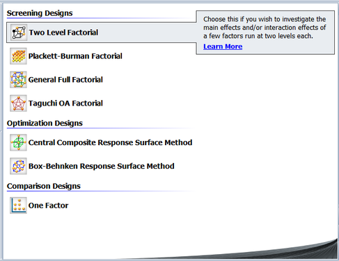
The factorial experiments, where all combination of the levels of the factors are run, are usually referred to as full factorial experiments. Full factorial two level experiments are also referred to as [math]\displaystyle{ {2}^{k}\,\! }[/math] designs where [math]\displaystyle{ k\,\! }[/math] denotes the number of factors being investigated in the experiment. In Weibull++ DOE folios, these designs are referred to as 2 Level Factorial Designs as shown in the figure below.
A full factorial two level design with [math]\displaystyle{ k\,\! }[/math] factors requires [math]\displaystyle{ {{2}^{k}}\,\! }[/math] runs for a single replicate. For example, a two level experiment with three factors will require [math]\displaystyle{ 2\times 2\times 2={{2}^{3}}=8\,\! }[/math] runs. The choice of the two levels of factors used in two level experiments depends on the factor; some factors naturally have two levels. For example, if gender is a factor, then male and female are the two levels. For other factors, the limits of the range of interest are usually used. For example, if temperature is a factor that varies from [math]\displaystyle{ {45}^{o}C\,\! }[/math] to [math]\displaystyle{ {90}^{o}C\,\! }[/math], then the two levels used in the [math]\displaystyle{ {2}^{k}\,\! }[/math] design for this factor would be [math]\displaystyle{ {45}^{o}\,\!C\,\! }[/math] and [math]\displaystyle{ {90}^{o}\,\!C\,\! }[/math].
The two levels of the factor in the [math]\displaystyle{ {2}^{k}\,\! }[/math] design are usually represented as [math]\displaystyle{ -1\,\! }[/math] (for the first level) and [math]\displaystyle{ 1\,\! }[/math] (for the second level). Note that this representation is reversed from the coding used in General Full Factorial Designs for the indicator variables that represent two level factors in ANOVA models. For ANOVA models, the first level of the factor was represented using a value of [math]\displaystyle{ 1\,\! }[/math] for the indicator variable, while the second level was represented using a value of [math]\displaystyle{ -1\,\! }[/math]. For details on the notation used for two level experiments refer to Notation.
The 22 Design
The simplest of the two level factorial experiments is the [math]\displaystyle{ {2}^{2}\,\! }[/math] design where two factors (say factor [math]\displaystyle{ A\,\! }[/math] and factor [math]\displaystyle{ B\,\! }[/math]) are investigated at two levels. A single replicate of this design will require four runs ([math]\displaystyle{ {{2}^{2}}=2\times 2=4\,\! }[/math]) The effects investigated by this design are the two main effects, [math]\displaystyle{ A\,\! }[/math] and [math]\displaystyle{ B,\,\! }[/math] and the interaction effect [math]\displaystyle{ AB\,\! }[/math]. The treatments for this design are shown in figure (a) below. In figure (a), letters are used to represent the treatments. The presence of a letter indicates the high level of the corresponding factor and the absence indicates the low level. For example, (1) represents the treatment combination where all factors involved are at the low level or the level represented by [math]\displaystyle{ -1\,\! }[/math] ; [math]\displaystyle{ a\,\! }[/math] represents the treatment combination where factor [math]\displaystyle{ A\,\! }[/math] is at the high level or the level of [math]\displaystyle{ 1\,\! }[/math], while the remaining factors (in this case, factor [math]\displaystyle{ B\,\! }[/math]) are at the low level or the level of [math]\displaystyle{ -1\,\! }[/math]. Similarly, [math]\displaystyle{ b\,\! }[/math] represents the treatment combination where factor [math]\displaystyle{ B\,\! }[/math] is at the high level or the level of [math]\displaystyle{ 1\,\! }[/math], while factor [math]\displaystyle{ A\,\! }[/math] is at the low level and [math]\displaystyle{ ab\,\! }[/math] represents the treatment combination where factors [math]\displaystyle{ A\,\! }[/math] and [math]\displaystyle{ B\,\! }[/math] are at the high level or the level of the 1. Figure (b) below shows the design matrix for the [math]\displaystyle{ {2}^{2}\,\! }[/math] design. It can be noted that the sum of the terms resulting from the product of any two columns of the design matrix is zero. As a result the [math]\displaystyle{ {2}^{2}\,\! }[/math] design is an orthogonal design. In fact, all [math]\displaystyle{ {2}^{k}\,\! }[/math] designs are orthogonal designs. This property of the [math]\displaystyle{ {2}^{k}\,\! }[/math] designs offers a great advantage in the analysis because of the simplifications that result from orthogonality. These simplifications are explained later on in this chapter. The [math]\displaystyle{ {2}^{2}\,\! }[/math] design can also be represented geometrically using a square with the four treatment combinations lying at the four corners, as shown in figure (c) below.
The 23 Design
The [math]\displaystyle{ {2}^{3}\,\! }[/math] design is a two level factorial experiment design with three factors (say factors [math]\displaystyle{ A\,\! }[/math], [math]\displaystyle{ B\,\! }[/math] and [math]\displaystyle{ C\,\! }[/math]). This design tests three ([math]\displaystyle{ k=3\,\! }[/math]) main effects, [math]\displaystyle{ A\,\! }[/math], [math]\displaystyle{ B\,\! }[/math] and [math]\displaystyle{ C\,\! }[/math] ; three ([math]\displaystyle{ (_{2}^{k})=\,\! }[/math] [math]\displaystyle{ (_{2}^{3})=3\,\! }[/math]) two factor interaction effects, [math]\displaystyle{ AB\,\! }[/math], [math]\displaystyle{ BC\,\! }[/math], [math]\displaystyle{ AC\,\! }[/math] ; and one ([math]\displaystyle{ (_{3}^{k})=\,\! }[/math] [math]\displaystyle{ (_{3}^{3})=1\,\! }[/math]) three factor interaction effect, [math]\displaystyle{ ABC\,\! }[/math]. The design requires eight runs per replicate. The eight treatment combinations corresponding to these runs are [math]\displaystyle{ (1)\,\! }[/math], [math]\displaystyle{ a\,\! }[/math], [math]\displaystyle{ b\,\! }[/math], [math]\displaystyle{ ab\,\! }[/math], [math]\displaystyle{ c\,\! }[/math], [math]\displaystyle{ ac\,\! }[/math], [math]\displaystyle{ bc\,\! }[/math] and [math]\displaystyle{ abc\,\! }[/math]. Note that the treatment combinations are written in such an order that factors are introduced one by one with each new factor being combined with the preceding terms. This order of writing the treatments is called the standard order or Yates' order. The [math]\displaystyle{ {2}^{3}\,\! }[/math] design is shown in figure (a) below. The design matrix for the [math]\displaystyle{ {2}^{3}\,\! }[/math] design is shown in figure (b). The design matrix can be constructed by following the standard order for the treatment combinations to obtain the columns for the main effects and then multiplying the main effects columns to obtain the interaction columns.
The [math]\displaystyle{ {2}^{3}\,\! }[/math] design can also be represented geometrically using a cube with the eight treatment combinations lying at the eight corners as shown in the figure above.
Analysis of 2k Designs
The [math]\displaystyle{ {2}^{k}\,\! }[/math] designs are a special category of the factorial experiments where all the factors are at two levels. The fact that these designs contain factors at only two levels and are orthogonal greatly simplifies their analysis even when the number of factors is large. The use of [math]\displaystyle{ {2}^{k}\,\! }[/math] designs in investigating a large number of factors calls for a revision of the notation used previously for the ANOVA models. The case for revised notation is made stronger by the fact that the ANOVA and multiple linear regression models are identical for [math]\displaystyle{ {2}^{k}\,\! }[/math] designs because all factors are only at two levels. Therefore, the notation of the regression models is applied to the ANOVA models for these designs, as explained next.
Notation
Based on the notation used in General Full Factorial Designs, the ANOVA model for a two level factorial experiment with three factors would be as follows:
- [math]\displaystyle{ \begin{align} & Y= & \mu +{{\tau }_{1}}\cdot {{x}_{1}}+{{\delta }_{1}}\cdot {{x}_{2}}+{{(\tau \delta )}_{11}}\cdot {{x}_{1}}{{x}_{2}}+{{\gamma }_{1}}\cdot {{x}_{3}} \\ & & +{{(\tau \gamma )}_{11}}\cdot {{x}_{1}}{{x}_{3}}+{{(\delta \gamma )}_{11}}\cdot {{x}_{2}}{{x}_{3}}+{{(\tau \delta \gamma )}_{111}}\cdot {{x}_{1}}{{x}_{2}}{{x}_{3}}+\epsilon \end{align}\,\! }[/math]
where:
- • [math]\displaystyle{ \mu \,\! }[/math] represents the overall mean
- • [math]\displaystyle{ {{\tau }_{1}}\,\! }[/math] represents the independent effect of the first factor (factor [math]\displaystyle{ A\,\! }[/math]) out of the two effects [math]\displaystyle{ {{\tau }_{1}}\,\! }[/math] and [math]\displaystyle{ {{\tau }_{2}}\,\! }[/math]
- • [math]\displaystyle{ {{\delta }_{1}}\,\! }[/math] represents the independent effect of the second factor (factor [math]\displaystyle{ B\,\! }[/math]) out of the two effects [math]\displaystyle{ {{\delta }_{1}}\,\! }[/math] and [math]\displaystyle{ {{\delta }_{2}}\,\! }[/math]
- • [math]\displaystyle{ {{(\tau \delta )}_{11}}\,\! }[/math] represents the independent effect of the interaction [math]\displaystyle{ AB\,\! }[/math] out of the other interaction effects
- • [math]\displaystyle{ {{\gamma }_{1}}\,\! }[/math] represents the effect of the third factor (factor [math]\displaystyle{ C\,\! }[/math]) out of the two effects [math]\displaystyle{ {{\gamma }_{1}}\,\! }[/math] and [math]\displaystyle{ {{\gamma }_{2}}\,\! }[/math]
- • [math]\displaystyle{ {{(\tau \gamma )}_{11}}\,\! }[/math] represents the effect of the interaction [math]\displaystyle{ AC\,\! }[/math] out of the other interaction effects
- • [math]\displaystyle{ {{(\delta \gamma )}_{11}}\,\! }[/math] represents the effect of the interaction [math]\displaystyle{ BC\,\! }[/math] out of the other interaction effects
- • [math]\displaystyle{ {{(\tau \delta \gamma )}_{111}}\,\! }[/math] represents the effect of the interaction [math]\displaystyle{ ABC\,\! }[/math] out of the other interaction effects
and [math]\displaystyle{ \epsilon \,\! }[/math] is the random error term.
The notation for a linear regression model having three predictor variables with interactions is:
- [math]\displaystyle{ \begin{align} & Y= & {{\beta }_{0}}+{{\beta }_{1}}\cdot {{x}_{1}}+{{\beta }_{2}}\cdot {{x}_{2}}+{{\beta }_{12}}\cdot {{x}_{1}}{{x}_{2}}+{{\beta }_{3}}\cdot {{x}_{3}} \\ & & +{{\beta }_{13}}\cdot {{x}_{1}}{{x}_{3}}+{{\beta }_{23}}\cdot {{x}_{2}}{{x}_{3}}+{{\beta }_{123}}\cdot {{x}_{1}}{{x}_{2}}{{x}_{3}}+\epsilon \end{align}\,\! }[/math]
The notation for the regression model is much more convenient, especially for the case when a large number of higher order interactions are present. In two level experiments, the ANOVA model requires only one indicator variable to represent each factor for both qualitative and quantitative factors. Therefore, the notation for the multiple linear regression model can be applied to the ANOVA model of the experiment that has all the factors at two levels. For example, for the experiment of the ANOVA model given above, [math]\displaystyle{ {{\beta }_{0}}\,\! }[/math] can represent the overall mean instead of [math]\displaystyle{ \mu \,\! }[/math], and [math]\displaystyle{ {{\beta }_{1}}\,\! }[/math] can represent the independent effect, [math]\displaystyle{ {{\tau }_{1}}\,\! }[/math], of factor [math]\displaystyle{ A\,\! }[/math]. Other main effects can be represented in a similar manner. The notation for the interaction effects is much more simplified (e.g., [math]\displaystyle{ {{\beta }_{123}}\,\! }[/math] can be used to represent the three factor interaction effect, [math]\displaystyle{ {{(\tau \beta \gamma )}_{111}}\,\! }[/math]).
As mentioned earlier, it is important to note that the coding for the indicator variables for the ANOVA models of two level factorial experiments is reversed from the coding followed in General Full Factorial Designs. Here [math]\displaystyle{ -1\,\! }[/math] represents the first level of the factor while [math]\displaystyle{ 1\,\! }[/math] represents the second level. This is because for a two level factor a single variable is needed to represent the factor for both qualitative and quantitative factors. For quantitative factors, using [math]\displaystyle{ -1\,\! }[/math] for the first level (which is the low level) and 1 for the second level (which is the high level) keeps the coding consistent with the numerical value of the factors. The change in coding between the two coding schemes does not affect the analysis except that signs of the estimated effect coefficients will be reversed (i.e., numerical values of [math]\displaystyle{ {{\hat{\tau }}_{1}}\,\! }[/math], obtained based on the coding of General Full Factorial Designs, and [math]\displaystyle{ {{\hat{\beta }}_{1}}\,\! }[/math], obtained based on the new coding, will be the same but their signs would be opposite).
- [math]\displaystyle{ \begin{align} & & \text{Factor }A\text{ Coding (two level factor)} \\ & & \end{align}\,\! }[/math]
- [math]\displaystyle{ \begin{matrix} \text{Previous Coding} & {} & {} & {} & \text{Coding for }{{\text{2}}^{k}}\text{ Designs} \\ {} & {} & {} & {} & {} \\ Effect\text{ }{{\tau }_{1}}\ \ :\ \ {{x}_{1}}=1\text{ } & {} & {} & {} & Effect\text{ }{{\tau }_{1}}\text{ (or }-{{\beta }_{1}}\text{)}\ \ :\ \ {{x}_{1}}=-1\text{ } \\ Effect\text{ }{{\tau }_{2}}\ \ :\ \ {{x}_{1}}=-1\text{ } & {} & {} & {} & Effect\text{ }{{\tau }_{2}}\text{ (or }{{\beta }_{1}}\text{)}\ \ :\ \ {{x}_{1}}=1\text{ } \\ \end{matrix}\,\! }[/math]
In summary, the ANOVA model for the experiments with all factors at two levels is different from the ANOVA models for other experiments in terms of the notation in the following two ways:
- • The notation of the regression models is used for the effect coefficients.
- • The coding of the indicator variables is reversed.
Special Features
Consider the design matrix, [math]\displaystyle{ X\,\! }[/math], for the [math]\displaystyle{ {2}^{3}\,\! }[/math] design discussed above. The ([math]\displaystyle{ {{X}^{\prime }}X\,\! }[/math]) [math]\displaystyle{ ^{-1}\,\! }[/math] matrix is:
Notice that, due to the orthogonal design of the [math]\displaystyle{ X\,\! }[/math] matrix, the [math]\displaystyle{ {{({{X}^{\prime }}X)}^{-1}}\,\! }[/math] has been simplified to a diagonal matrix which can be written as:
- [math]\displaystyle{ \begin{align} {{({{X}^{\prime }}X)}^{-1}}= & 0.125\cdot I = & \frac{1}{8}\cdot I = & \frac{1}{{{2}^{3}}}\cdot I \end{align}\,\! }[/math]
where [math]\displaystyle{ I\,\! }[/math] represents the identity matrix of the same order as the design matrix, [math]\displaystyle{ X\,\! }[/math]. Since there are eight observations per replicate of the [math]\displaystyle{ {2}^{3}\,\! }[/math] design, the [math]\displaystyle{ (X\,\! }[/math] ' [math]\displaystyle{ X{{)}^{-1}}\,\! }[/math] matrix for [math]\displaystyle{ m\,\! }[/math] replicates of this design can be written as:
- [math]\displaystyle{ {{({{X}^{\prime }}X)}^{-1}}=\frac{1}{({{2}^{3}}\cdot m)}\cdot I\,\! }[/math]
The [math]\displaystyle{ {{({{X}^{\prime }}X)}^{-1}}\,\! }[/math] matrix for any [math]\displaystyle{ {2}^{k}\,\! }[/math] design can now be written as:
- [math]\displaystyle{ {{({{X}^{\prime }}X)}^{-1}}=\frac{1}{({{2}^{k}}\cdot m)}\cdot I\,\! }[/math]
Then the variance-covariance matrix for the [math]\displaystyle{ {2}^{k}\,\! }[/math] design is:
- [math]\displaystyle{ \begin{align} C= & {{{\hat{\sigma }}}^{2}}\cdot {{({{X}^{\prime }}X)}^{-1}} = & M{{S}_{E}}\cdot {{({{X}^{\prime }}X)}^{-1}} = & \frac{M{{S}_{E}}}{({{2}^{k}}\cdot m)}\cdot I \end{align}\,\! }[/math]
Note that the variance-covariance matrix for the [math]\displaystyle{ {2}^{k}\,\! }[/math] design is also a diagonal matrix. Therefore, the estimated effect coefficients ([math]\displaystyle{ {{\beta }_{1}}\,\! }[/math], [math]\displaystyle{ {{\beta }_{2}}\,\! }[/math], [math]\displaystyle{ {{\beta }_{12}},\,\! }[/math] etc.) for these designs are uncorrelated. This implies that the terms in the [math]\displaystyle{ {2}^{k}\,\! }[/math] design (main effects, interactions) are independent of each other. Consequently, the extra sum of squares for each of the terms in these designs is independent of the sequence of terms in the model, and also independent of the presence of other terms in the model. As a result the sequential and partial sum of squares for the terms are identical for these designs and will always add up to the model sum of squares. Multicollinearity is also not an issue for these designs.
It can also be noted from the equation given above, that in addition to the [math]\displaystyle{ C\,\! }[/math] matrix being diagonal, all diagonal elements of the [math]\displaystyle{ C\,\! }[/math] matrix are identical. This means that the variance (or its square root, the standard error) of all estimated effect coefficients are the same. The standard error, [math]\displaystyle{ se({{\hat{\beta }}_{j}})\,\! }[/math], for all the coefficients is:
- [math]\displaystyle{ \begin{align} se({{{\hat{\beta }}}_{j}})= & \sqrt{{{C}_{jj}}} = & \sqrt{\frac{M{{S}_{E}}}{({{2}^{k}}\cdot m)}}\text{ }for\text{ }all\text{ }j \end{align}\,\! }[/math]
This property is used to construct the normal probability plot of effects in [math]\displaystyle{ {2}^{k}\,\! }[/math] designs and identify significant effects using graphical techniques. For details on the normal probability plot of effects in a Weibull++ DOE folio, refer to Normal Probability Plot of Effects.
Example
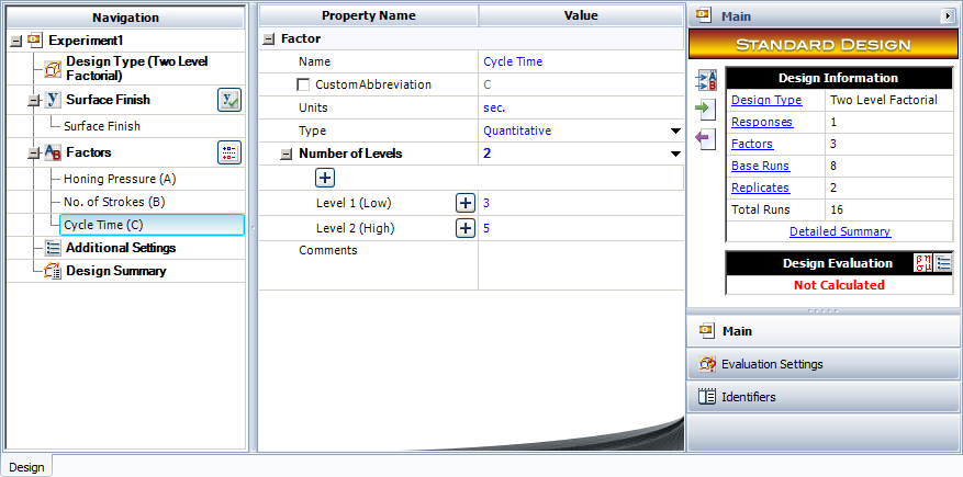
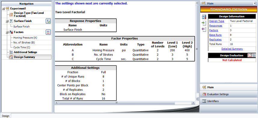
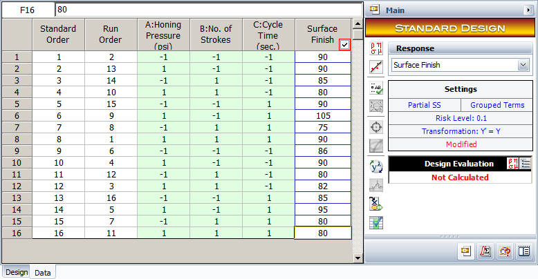
To illustrate the analysis of a full factorial [math]\displaystyle{ {2}^{k}\,\! }[/math] design, consider a three factor experiment to investigate the effect of honing pressure, number of strokes and cycle time on the surface finish of automobile brake drums. Each of these factors is investigated at two levels. The honing pressure is investigated at levels of 200 [math]\displaystyle{ psi\,\! }[/math] and 400 [math]\displaystyle{ psi\,\! }[/math], the number of strokes used is 3 and 5 and the two levels of the cycle time are 3 and 5 seconds. The design for this experiment is set up in a Weibull++ DOE folio as shown in the first two following figures. It is decided to run two replicates for this experiment. The surface finish data collected from each run (using randomization) and the complete design is shown in the third following figure. The analysis of the experiment data is explained next.
The applicable model using the notation for [math]\displaystyle{ {2}^{k}\,\! }[/math] designs is:
- [math]\displaystyle{ \begin{align} Y= & {{\beta }_{0}}+{{\beta }_{1}}\cdot {{x}_{1}}+{{\beta }_{2}}\cdot {{x}_{2}}+{{\beta }_{12}}\cdot {{x}_{1}}{{x}_{2}}+{{\beta }_{3}}\cdot {{x}_{3}} \\ & +{{\beta }_{13}}\cdot {{x}_{1}}{{x}_{3}}+{{\beta }_{23}}\cdot {{x}_{2}}{{x}_{3}}+{{\beta }_{123}}\cdot {{x}_{1}}{{x}_{2}}{{x}_{3}}+\epsilon \end{align}\,\! }[/math]
where the indicator variable, [math]\displaystyle{ {{x}_{1,}}\,\! }[/math] represents factor [math]\displaystyle{ A\,\! }[/math] (honing pressure), [math]\displaystyle{ {{x}_{1}}=-1\,\! }[/math] represents the low level of 200 [math]\displaystyle{ psi\,\! }[/math] and [math]\displaystyle{ {{x}_{1}}=1\,\! }[/math] represents the high level of 400 [math]\displaystyle{ psi\,\! }[/math]. Similarly, [math]\displaystyle{ {{x}_{2}}\,\! }[/math] and [math]\displaystyle{ {{x}_{3}}\,\! }[/math] represent factors [math]\displaystyle{ B\,\! }[/math] (number of strokes) and [math]\displaystyle{ C\,\! }[/math] (cycle time), respectively. [math]\displaystyle{ {{\beta }_{0}}\,\! }[/math] is the overall mean, while [math]\displaystyle{ {{\beta }_{1}}\,\! }[/math], [math]\displaystyle{ {{\beta }_{2}}\,\! }[/math] and [math]\displaystyle{ {{\beta }_{3}}\,\! }[/math] are the effect coefficients for the main effects of factors [math]\displaystyle{ A\,\! }[/math], [math]\displaystyle{ B\,\! }[/math] and [math]\displaystyle{ C\,\! }[/math], respectively. [math]\displaystyle{ {{\beta }_{12}}\,\! }[/math], [math]\displaystyle{ {{\beta }_{13}}\,\! }[/math] and [math]\displaystyle{ {{\beta }_{23}}\,\! }[/math] are the effect coefficients for the [math]\displaystyle{ AB\,\! }[/math], [math]\displaystyle{ AC\,\! }[/math] and [math]\displaystyle{ BC\,\! }[/math] interactions, while [math]\displaystyle{ {{\beta }_{123}}\,\! }[/math] represents the [math]\displaystyle{ ABC\,\! }[/math] interaction.
If the subscripts for the run ([math]\displaystyle{ i\,\! }[/math] ; [math]\displaystyle{ i=\,\! }[/math] 1 to 8) and replicates ([math]\displaystyle{ j\,\! }[/math] ; [math]\displaystyle{ j=\,\! }[/math] 1,2) are included, then the model can be written as:
- [math]\displaystyle{ \begin{align} {{Y}_{ij}}= & {{\beta }_{0}}+{{\beta }_{1}}\cdot {{x}_{ij1}}+{{\beta }_{2}}\cdot {{x}_{ij2}}+{{\beta }_{12}}\cdot {{x}_{ij1}}{{x}_{ij2}}+{{\beta }_{3}}\cdot {{x}_{ij3}} \\ & +{{\beta }_{13}}\cdot {{x}_{ij1}}{{x}_{ij3}}+{{\beta }_{23}}\cdot {{x}_{ij2}}{{x}_{ij3}}+{{\beta }_{123}}\cdot {{x}_{ij1}}{{x}_{ij2}}{{x}_{ij3}}+{{\epsilon }_{ij}} \end{align}\,\! }[/math]
To investigate how the given factors affect the response, the following hypothesis tests need to be carried:
- [math]\displaystyle{ {{H}_{0}}\ \ :\ \ {{\beta }_{1}}=0\,\! }[/math]
- [math]\displaystyle{ {{H}_{1}}\ \ :\ \ {{\beta }_{1}}\ne 0\,\! }[/math]
This test investigates the main effect of factor [math]\displaystyle{ A\,\! }[/math] (honing pressure). The statistic for this test is:
- [math]\displaystyle{ {{({{F}_{0}})}_{A}}=\frac{M{{S}_{A}}}{M{{S}_{E}}}\,\! }[/math]
where [math]\displaystyle{ M{{S}_{A}}\,\! }[/math] is the mean square for factor [math]\displaystyle{ A\,\! }[/math] and [math]\displaystyle{ M{{S}_{E}}\,\! }[/math] is the error mean square. Hypotheses for the other main effects, [math]\displaystyle{ B\,\! }[/math] and [math]\displaystyle{ C\,\! }[/math], can be written in a similar manner.
- [math]\displaystyle{ {{H}_{0}}\ \ :\ \ {{\beta }_{12}}=0\,\! }[/math]
- [math]\displaystyle{ {{H}_{1}}\ \ :\ \ {{\beta }_{12}}\ne 0\,\! }[/math]
This test investigates the two factor interaction [math]\displaystyle{ AB\,\! }[/math]. The statistic for this test is:
- [math]\displaystyle{ {{({{F}_{0}})}_{AB}}=\frac{M{{S}_{AB}}}{M{{S}_{E}}}\,\! }[/math]
where [math]\displaystyle{ M{{S}_{AB}}\,\! }[/math] is the mean square for the interaction [math]\displaystyle{ AB\,\! }[/math] and [math]\displaystyle{ M{{S}_{E}}\,\! }[/math] is the error mean square. Hypotheses for the other two factor interactions, [math]\displaystyle{ AC\,\! }[/math] and [math]\displaystyle{ BC\,\! }[/math], can be written in a similar manner.
- [math]\displaystyle{ {{H}_{0}}\ \ :\ \ {{\beta }_{123}}=0\,\! }[/math]
- [math]\displaystyle{ {{H}_{1}}\ \ :\ \ {{\beta }_{123}}\ne 0\,\! }[/math]
This test investigates the three factor interaction [math]\displaystyle{ ABC\,\! }[/math]. The statistic for this test is:
- [math]\displaystyle{ {{({{F}_{0}})}_{ABC}}=\frac{M{{S}_{ABC}}}{M{{S}_{E}}}\,\! }[/math]
where [math]\displaystyle{ M{{S}_{ABC}}\,\! }[/math] is the mean square for the interaction [math]\displaystyle{ ABC\,\! }[/math] and [math]\displaystyle{ M{{S}_{E}}\,\! }[/math] is the error mean square. To calculate the test statistics, it is convenient to express the ANOVA model in the form [math]\displaystyle{ y=X\beta +\epsilon \,\! }[/math].
Expression of the ANOVA Model as [math]\displaystyle{ y=X\beta +\epsilon \,\! }[/math]
In matrix notation, the ANOVA model can be expressed as:
- [math]\displaystyle{ y=X\beta +\epsilon \,\! }[/math]
where:
Calculation of the Extra Sum of Squares for the Factors
Knowing the matrices [math]\displaystyle{ y\,\! }[/math], [math]\displaystyle{ X\,\! }[/math] and [math]\displaystyle{ \beta \,\! }[/math], the extra sum of squares for the factors can be calculated. These are used to calculate the mean squares that are used to obtain the test statistics. Since the experiment design is orthogonal, the partial and sequential extra sum of squares are identical. The extra sum of squares for each effect can be calculated as shown next. As an example, the extra sum of squares for the main effect of factor [math]\displaystyle{ A\,\! }[/math] is:
- [math]\displaystyle{ \begin{align} S{{S}_{A}}= & Model\text{ }Sum\text{ }of\text{ }Squares - Sum\text{ }of\text{ }Squares\text{ }of\text{ }model\text{ }excluding\text{ }the\text{ }main\text{ }effect\text{ }of\text{ }A \\ = & {{y}^{\prime }}[H-(1/16)J]y-{{y}^{\prime }}[{{H}_{\tilde{\ }A}}-(1/16)J]y \end{align}\,\! }[/math]
where [math]\displaystyle{ H\,\! }[/math] is the hat matrix and [math]\displaystyle{ J\,\! }[/math] is the matrix of ones. The matrix [math]\displaystyle{ {{H}_{\tilde{\ }A}}\,\! }[/math] can be calculated using [math]\displaystyle{ {{H}_{\tilde{\ }A}}={{X}_{\tilde{\ }A}}{{(X_{\tilde{\ }A}^{\prime }{{X}_{\tilde{\ }A}})}^{-1}}X_{\tilde{\ }A}^{\prime }\,\! }[/math] where [math]\displaystyle{ {{X}_{\tilde{\ }A}}\,\! }[/math] is the design matrix, [math]\displaystyle{ X\,\! }[/math], excluding the second column that represents the main effect of factor [math]\displaystyle{ A\,\! }[/math]. Thus, the sum of squares for the main effect of factor [math]\displaystyle{ A\,\! }[/math] is:
- [math]\displaystyle{ \begin{align} S{{S}_{A}}= & {{y}^{\prime }}[H-(1/16)J]y-{{y}^{\prime }}[{{H}_{\tilde{\ }A}}-(1/16)J]y \\ = & 654.4375-549.375 \\ = & 105.0625 \end{align}\,\! }[/math]
Similarly, the extra sum of squares for the interaction effect [math]\displaystyle{ AB\,\! }[/math] is:
- [math]\displaystyle{ \begin{align} S{{S}_{AB}}= & {{y}^{\prime }}[H-(1/16)J]y-{{y}^{\prime }}[{{H}_{\tilde{\ }AB}}-(1/16)J]y \\ = & 654.4375-636.375 \\ = & 18.0625 \end{align}\,\! }[/math]
The extra sum of squares for other effects can be obtained in a similar manner.
Calculation of the Test Statistics
Knowing the extra sum of squares, the test statistic for the effects can be calculated. For example, the test statistic for the interaction [math]\displaystyle{ AB\,\! }[/math] is:
- [math]\displaystyle{ \begin{align} {{({{f}_{0}})}_{AB}}= & \frac{M{{S}_{AB}}}{M{{S}_{E}}} \\ = & \frac{S{{S}_{AB}}/dof(S{{S}_{AB}})}{S{{S}_{E}}/dof(S{{S}_{E}})} \\ = & \frac{18.0625/1}{147.5/8} \\ = & 0.9797 \end{align}\,\! }[/math]
where [math]\displaystyle{ M{{S}_{AB}}\,\! }[/math] is the mean square for the [math]\displaystyle{ AB\,\! }[/math] interaction and [math]\displaystyle{ M{{S}_{E}}\,\! }[/math] is the error mean square. The [math]\displaystyle{ p\,\! }[/math] value corresponding to the statistic, [math]\displaystyle{ {{({{f}_{0}})}_{AB}}=0.9797\,\! }[/math], based on the [math]\displaystyle{ F\,\! }[/math] distribution with one degree of freedom in the numerator and eight degrees of freedom in the denominator is:
- [math]\displaystyle{ \begin{align} p\text{ }value= & 1-P(F\le {{({{f}_{0}})}_{AB}}) \\ = & 1-0.6487 \\ = & 0.3513 \end{align}\,\! }[/math]
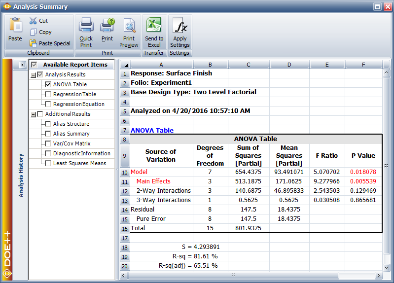
Assuming that the desired significance is 0.1, since [math]\displaystyle{ p\,\! }[/math] value > 0.1, it can be concluded that the interaction between honing pressure and number of strokes does not affect the surface finish of the brake drums. Tests for other effects can be carried out in a similar manner. The results are shown in the ANOVA Table in the following figure. The values S, R-sq and R-sq(adj) in the figure indicate how well the model fits the data. The value of S represents the standard error of the model, R-sq represents the coefficient of multiple determination and R-sq(adj) represents the adjusted coefficient of multiple determination. For details on these values refer to Multiple Linear Regression Analysis.
Calculation of Effect Coefficients
The estimate of effect coefficients can also be obtained:
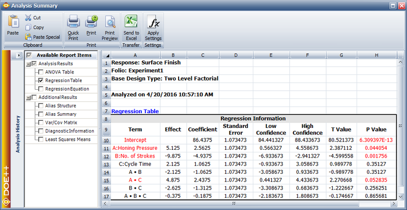
The coefficients and related results are shown in the Regression Information table above. In the table, the Effect column displays the effects, which are simply twice the coefficients. The Standard Error column displays the standard error, [math]\displaystyle{ se({{\hat{\beta }}_{j}})\,\! }[/math]. The Low CI and High CI columns display the confidence interval on the coefficients. The interval shown is the 90% interval as the significance is chosen as 0.1. The T Value column displays the [math]\displaystyle{ t\,\! }[/math] statistic, [math]\displaystyle{ {{t}_{0}}\,\! }[/math], corresponding to the coefficients. The P Value column displays the [math]\displaystyle{ p\,\! }[/math] value corresponding to the [math]\displaystyle{ t\,\! }[/math] statistic. (For details on how these results are calculated, refer to General Full Factorial Designs). Plots of residuals can also be obtained from the DOE folio to ensure that the assumptions related to the ANOVA model are not violated.
Model Equation
From the analysis results in the above figure within calculation of effect coefficients section, it is seen that effects [math]\displaystyle{ A\,\! }[/math], [math]\displaystyle{ B\,\! }[/math] and [math]\displaystyle{ AC\,\! }[/math] are significant. In a DOE folio, the [math]\displaystyle{ p\,\! }[/math] values for the significant effects are displayed in red in the ANOVA Table for easy identification. Using the values of the estimated effect coefficients, the model for the present [math]\displaystyle{ {2}^{3}\,\! }[/math] design in terms of the coded values can be written as:
- [math]\displaystyle{ \begin{align} \hat{y}= & {{\beta }_{0}}+{{\beta }_{1}}\cdot {{x}_{1}}+{{\beta }_{2}}\cdot {{x}_{2}}+{{\beta }_{13}}\cdot {{x}_{1}}{{x}_{3}} \\ = & 86.4375+2.5625{{x}_{1}}-4.9375{{x}_{2}}+2.4375{{x}_{1}}{{x}_{3}} \end{align}\,\! }[/math]
To make the model hierarchical, the main effect, [math]\displaystyle{ C\,\! }[/math], needs to be included in the model (because the interaction [math]\displaystyle{ AC\,\! }[/math] is included in the model). The resulting model is:
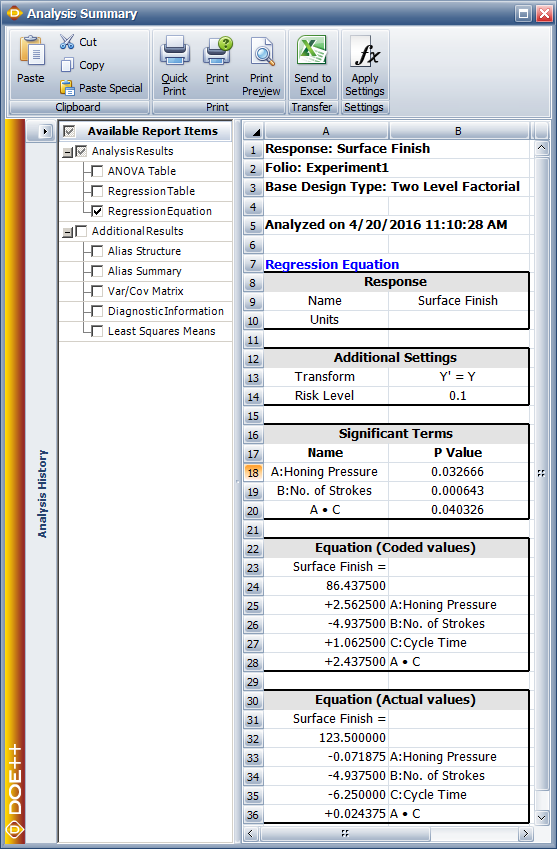
- [math]\displaystyle{ \hat{y}=86.4375+2.5625{{x}_{1}}-4.9375{{x}_{2}}+1.0625{{x}_{3}}+2.4375{{x}_{1}}{{x}_{3}}\,\! }[/math]
This equation can be viewed in a DOE folio, as shown in the following figure, using the Show Analysis Summary icon in the Control Panel. The equation shown in the figure will match the hierarchical model once the required terms are selected using the Select Effects icon.
Replicated and Repeated Runs
In the case of replicated experiments, it is important to note the difference between replicated runs and repeated runs. Both repeated and replicated runs are multiple response readings taken at the same factor levels. However, repeated runs are response observations taken at the same time or in succession. Replicated runs are response observations recorded in a random order. Therefore, replicated runs include more variation than repeated runs. For example, a baker, who wants to investigate the effect of two factors on the quality of cakes, will have to bake four cakes to complete one replicate of a [math]\displaystyle{ {2}^{2}\,\! }[/math] design. Assume that the baker bakes eight cakes in all. If, for each of the four treatments of the [math]\displaystyle{ {2}^{2}\,\! }[/math] design, the baker selects one treatment at random and then bakes two cakes for this treatment at the same time then this is a case of two repeated runs. If, however, the baker bakes all the eight cakes randomly, then the eight cakes represent two sets of replicated runs. For repeated measurements, the average values of the response for each treatment should be entered into a DOE folio as shown in the following figure (a) when the two cakes for a particular treatment are baked together. For replicated measurements, when all the cakes are baked randomly, the data is entered as shown in the following figure (b).
Unreplicated 2k Designs
If a factorial experiment is run only for a single replicate then it is not possible to test hypotheses about the main effects and interactions as the error sum of squares cannot be obtained. This is because the number of observations in a single replicate equals the number of terms in the ANOVA model. Hence the model fits the data perfectly and no degrees of freedom are available to obtain the error sum of squares.
However, sometimes it is only possible to run a single replicate of the [math]\displaystyle{ {2}^{k}\,\! }[/math] design because of constraints on resources and time. In the absence of the error sum of squares, hypothesis tests to identify significant factors cannot be conducted. A number of methods of analyzing information obtained from unreplicated [math]\displaystyle{ {2}^{k}\,\! }[/math] designs are available. These include pooling higher order interactions, using the normal probability plot of effects or including center point replicates in the design.
Pooling Higher Order Interactions
One of the ways to deal with unreplicated [math]\displaystyle{ {2}^{k}\,\! }[/math] designs is to use the sum of squares of some of the higher order interactions as the error sum of squares provided these higher order interactions can be assumed to be insignificant. By dropping some of the higher order interactions from the model, the degrees of freedom corresponding to these interactions can be used to estimate the error mean square. Once the error mean square is known, the test statistics to conduct hypothesis tests on the factors can be calculated.
Normal Probability Plot of Effects
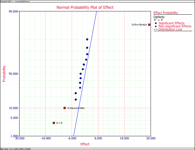
Another way to use unreplicated [math]\displaystyle{ {2}^{k}\,\! }[/math] designs to identify significant effects is to construct the normal probability plot of the effects. As mentioned in Special Features, the standard error for all effect coefficients in the [math]\displaystyle{ {2}^{k}\,\! }[/math] designs is the same. Therefore, on a normal probability plot of effect coefficients, all non-significant effect coefficients (with [math]\displaystyle{ \beta =0\,\! }[/math]) will fall along the straight line representative of the normal distribution, N([math]\displaystyle{ 0,{{\sigma }^{2}}/({{2}^{k}}\cdot m)\,\! }[/math]). Effect coefficients that show large deviations from this line will be significant since they do not come from this normal distribution. Similarly, since effects [math]\displaystyle{ =2\times \,\! }[/math] effect coefficients, all non-significant effects will also follow a straight line on the normal probability plot of effects. For replicated designs, the Effects Probability plot of a DOE folio plots the normalized effect values (or the T Values) on the standard normal probability line, N(0,1). However, in the case of unreplicated [math]\displaystyle{ {2}^{k}\,\! }[/math] designs, [math]\displaystyle{ {{\sigma }^{2}}\,\! }[/math] remains unknown since [math]\displaystyle{ M{{S}_{E}}\,\! }[/math] cannot be obtained. Lenth's method is used in this case to estimate the variance of the effects. For details on Lenth's method, please refer to Montgomery (2001). The DOE folio then uses this variance value to plot effects along the N(0, Lenth's effect variance) line. The method is illustrated in the following example.
Example
Vinyl panels, used as instrument panels in a certain automobile, are seen to develop defects after a certain amount of time. To investigate the issue, it is decided to carry out a two level factorial experiment. Potential factors to be investigated in the experiment are vacuum rate (factor [math]\displaystyle{ A\,\! }[/math]), material temperature (factor [math]\displaystyle{ B\,\! }[/math]), element intensity (factor [math]\displaystyle{ C\,\! }[/math]) and pre-stretch (factor [math]\displaystyle{ D\,\! }[/math]). The two levels of the factors used in the experiment are as shown in below.
With a [math]\displaystyle{ {2}^{4}\,\! }[/math] design requiring 16 runs per replicate it is only feasible for the manufacturer to run a single replicate.
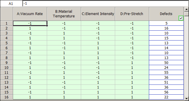
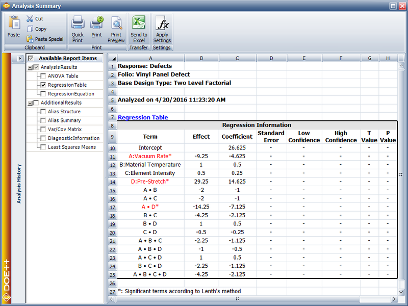
The experiment design and data, collected as percent defects, are shown in the following figure. Since the present experiment design contains only a single replicate, it is not possible to obtain an estimate of the error sum of squares, [math]\displaystyle{ S{{S}_{E}}\,\! }[/math]. It is decided to use the normal probability plot of effects to identify the significant effects. The effect values for each term are obtained as shown in the following figure.
Lenth's method uses these values to estimate the variance. As described in [Lenth, 1989], if all effects are arranged in ascending order, using their absolute values, then [math]\displaystyle{ {{s}_{0}}\,\! }[/math] is defined as 1.5 times the median value:
- [math]\displaystyle{ \begin{align} {{s}_{0}}= & 1.5\cdot median(\left| effect \right|) \\ = & 1.5\cdot 2 \\ = & 3 \end{align}\,\! }[/math]
Using [math]\displaystyle{ {{s}_{0}}\,\! }[/math], the "pseudo standard error" ([math]\displaystyle{ PSE\,\! }[/math]) is calculated as 1.5 times the median value of all effects that are less than 2.5 [math]\displaystyle{ {{s}_{0}}\,\! }[/math] :
- [math]\displaystyle{ \begin{align} PSE= & 1.5\cdot median(\left| effect \right|\ \ :\ \ \left| effect \right|\lt 2.5{{s}_{0}}) \\ = & 1.5\cdot 1.5 \\ = & 2.25 \end{align}\,\! }[/math]
Using [math]\displaystyle{ PSE\,\! }[/math] as an estimate of the effect variance, the effect variance is 2.25. Knowing the effect variance, the normal probability plot of effects for the present unreplicated experiment can be constructed as shown in the following figure. The line on this plot is the line N(0, 2.25). The plot shows that the effects [math]\displaystyle{ A\,\! }[/math], [math]\displaystyle{ D\,\! }[/math] and the interaction [math]\displaystyle{ AD\,\! }[/math] do not follow the distribution represented by this line. Therefore, these effects are significant.
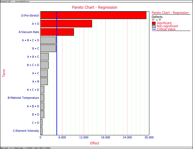
The significant effects can also be identified by comparing individual effect values to the margin of error or the threshold value using the pareto chart (see the third following figure). If the required significance is 0.1, then:
- [math]\displaystyle{ margin\text{ }of\text{ }error={{t}_{\alpha /2,d}}\cdot PSE\,\! }[/math]
The [math]\displaystyle{ t\,\! }[/math] statistic, [math]\displaystyle{ {{t}_{\alpha /2,d}}\,\! }[/math], is calculated at a significance of [math]\displaystyle{ \alpha /2\,\! }[/math] (for the two-sided hypothesis) and degrees of freedom [math]\displaystyle{ d=(\,\! }[/math] number of effects [math]\displaystyle{ )/3\,\! }[/math]. Thus:
- [math]\displaystyle{ \begin{align} margin\text{ }of\text{ }error= & {{t}_{0.05,5}}\cdot PSE \\ = & 2.015\cdot 2.25 \\ = & 4.534 \end{align}\,\! }[/math]
The value of 4.534 is shown as the critical value line in the third following figure. All effects with absolute values greater than the margin of error can be considered to be significant. These effects are [math]\displaystyle{ A\,\! }[/math], [math]\displaystyle{ D\,\! }[/math] and the interaction [math]\displaystyle{ AD\,\! }[/math]. Therefore, the vacuum rate, the pre-stretch and their interaction have a significant effect on the defects of the vinyl panels.
Center Point Replicates
Another method of dealing with unreplicated [math]\displaystyle{ {2}^{k}\,\! }[/math] designs that only have quantitative factors is to use replicated runs at the center point. The center point is the response corresponding to the treatment exactly midway between the two levels of all factors. Running multiple replicates at this point provides an estimate of pure error. Although running multiple replicates at any treatment level can provide an estimate of pure error, the other advantage of running center point replicates in the [math]\displaystyle{ {2}^{k}\,\! }[/math] design is in checking for the presence of curvature. The test for curvature investigates whether the model between the response and the factors is linear and is discussed in Center Pt. Replicates to Test Curvature.
Example: Use Center Point to Get Pure Error
Consider a [math]\displaystyle{ {2}^{2}\,\! }[/math] experiment design to investigate the effect of two factors, [math]\displaystyle{ A\,\! }[/math] and [math]\displaystyle{ B\,\! }[/math], on a certain response. The energy consumed when the treatments of the [math]\displaystyle{ {2}^{2}\,\! }[/math] design are run is considerably larger than the energy consumed for the center point run (because at the center point the factors are at their middle levels). Therefore, the analyst decides to run only a single replicate of the design and augment the design by five replicated runs at the center point as shown in the following figure. The design properties for this experiment are shown in the second following figure. The complete experiment design is shown in the third following figure. The center points can be used in the identification of significant effects as shown next.
Since the present [math]\displaystyle{ {2}^{2}\,\! }[/math] design is unreplicated, there are no degrees of freedom available to calculate the error sum of squares. By augmenting this design with five center points, the response values at the center points, [math]\displaystyle{ y_{i}^{c}\,\! }[/math], can be used to obtain an estimate of pure error, [math]\displaystyle{ S{{S}_{PE}}\,\! }[/math]. Let [math]\displaystyle{ {{\bar{y}}^{c}}\,\! }[/math] represent the average response for the five replicates at the center. Then:
- [math]\displaystyle{ S{{S}_{PE}}=Sum\text{ }of\text{ }Squares\text{ }for\text{ }center\text{ }points\,\! }[/math]
- [math]\displaystyle{ \begin{align} S{{S}_{PE}}= & \underset{i=1}{\overset{5}{\mathop{\sum }}}\,{{(y_{i}^{c}-{{{\bar{y}}}^{c}})}^{2}} \\ = & {{(25.2-25.26)}^{2}}+...+{{(25.3-25.26)}^{2}} \\ = & 0.052 \end{align}\,\! }[/math]
Then the corresponding mean square is:
- [math]\displaystyle{ \begin{align} M{{S}_{PE}}= & \frac{S{{S}_{PE}}}{degrees\text{ }of\text{ }freedom} \\ = & \frac{0.052}{5-1} \\ = & 0.013 \end{align}\,\! }[/math]
Alternatively, [math]\displaystyle{ M{{S}_{PE}}\,\! }[/math] can be directly obtained by calculating the variance of the response values at the center points:
- [math]\displaystyle{ \begin{align} M{{S}_{PE}}= & {{s}^{2}} \\ = & \frac{\underset{i=1}{\overset{5}{\mathop{\sum }}}\,{{(y_{i}^{c}-{{{\bar{y}}}^{c}})}^{2}}}{5-1} \end{align}\,\! }[/math]
Once [math]\displaystyle{ M{{S}_{PE}}\,\! }[/math] is known, it can be used as the error mean square, [math]\displaystyle{ M{{S}_{E}}\,\! }[/math], to carry out the test of significance for each effect. For example, to test the significance of the main effect of factor [math]\displaystyle{ A,\,\! }[/math] the sum of squares corresponding to this effect is obtained in the usual manner by considering only the four runs of the original [math]\displaystyle{ {2}^{2}\,\! }[/math] design.
- [math]\displaystyle{ \begin{align} S{{S}_{A}}= & {{y}^{\prime }}[H-(1/4)J]y-{{y}^{\prime }}[{{H}_{\tilde{\ }A}}-(1/4)J]y \\ = & 0.5625 \end{align}\,\! }[/math]
Then, the test statistic to test the significance of the main effect of factor [math]\displaystyle{ A\,\! }[/math] is:
- [math]\displaystyle{ \begin{align} {{({{f}_{0}})}_{A}}= & \frac{M{{S}_{A}}}{M{{S}_{E}}} \\ = & \frac{0.5625/1}{0.052/4} \\ = & 43.2692 \end{align}\,\! }[/math]
The [math]\displaystyle{ p\,\! }[/math] value corresponding to the statistic, [math]\displaystyle{ {{({{f}_{0}})}_{A}}=43.2692\,\! }[/math], based on the [math]\displaystyle{ F\,\! }[/math] distribution with one degree of freedom in the numerator and eight degrees of freedom in the denominator is:
- [math]\displaystyle{ \begin{align} p\text{ }value= & 1-P(F\le {{({{f}_{0}})}_{A}}) \\ = & 1-0.9972 \\ = & 0.0028 \end{align}\,\! }[/math]
Assuming that the desired significance is 0.1, since [math]\displaystyle{ p\,\! }[/math] value < 0.1, it can be concluded that the main effect of factor [math]\displaystyle{ A\,\! }[/math] significantly affects the response. This result is displayed in the ANOVA table as shown in the following figure. Test for the significance of other factors can be carried out in a similar manner.
Using Center Point Replicates to Test Curvature
Center point replicates can also be used to check for curvature in replicated or unreplicated [math]\displaystyle{ {2}^{k}\,\! }[/math] designs. The test for curvature investigates whether the model between the response and the factors is linear. The way the DOE folio handles center point replicates is similar to its handling of blocks. The center point replicates are treated as an additional factor in the model. The factor is labeled as Curvature in the results of the DOE folio. If Curvature turns out to be a significant factor in the results, then this indicates the presence of curvature in the model.
Example: Use Center Point to Test Curvature
To illustrate the use of center point replicates in testing for curvature, consider again the data of the single replicate [math]\displaystyle{ {2}^{2}\,\! }[/math] experiment from a preceding figure(labeled "[math]\displaystyle{ 2^2 }[/math] design augmented by five center point runs"). Let [math]\displaystyle{ {{x}_{1}}\,\! }[/math] be the indicator variable to indicate if the run is a center point:
- [math]\displaystyle{ \begin{matrix} {{x}_{1}}=0 & {} & \text{Center point run} \\ {{x}_{1}}=1 & {} & \text{Other run} \\ \end{matrix}\,\! }[/math]
If [math]\displaystyle{ {{x}_{2}}\,\! }[/math] and [math]\displaystyle{ {{x}_{3}}\,\! }[/math] are the indicator variables representing factors [math]\displaystyle{ A\,\! }[/math] and [math]\displaystyle{ B\,\! }[/math], respectively, then the model for this experiment is:
- [math]\displaystyle{ Y={{\beta }_{0}}+{{\beta }_{1}}\cdot {{x}_{1}}+{{\beta }_{2}}\cdot {{x}_{2}}+{{\beta }_{3}}\cdot {{x}_{3}}+{{\beta }_{23}}\cdot {{x}_{2}}{{x}_{3}}\,\! }[/math]
To investigate the presence of curvature, the following hypotheses need to be tested:
- [math]\displaystyle{ \begin{align} & {{H}_{0}}: & {{\beta }_{1}}=0\text{ (Curvature is absent)} \\ & {{H}_{1}}: & {{\beta }_{1}}\ne 0 \end{align}\,\! }[/math]
The test statistic to be used for this test is:
- [math]\displaystyle{ {{({{F}_{0}})}_{curvature}}=\frac{M{{S}_{curvature}}}{M{{S}_{E}}}\,\! }[/math]
where [math]\displaystyle{ M{{S}_{curvature}}\,\! }[/math] is the mean square for Curvature and [math]\displaystyle{ M{{S}_{E}}\,\! }[/math] is the error mean square.
Calculation of the Sum of Squares
The [math]\displaystyle{ X\,\! }[/math] matrix and [math]\displaystyle{ y\,\! }[/math] vector for this experiment are:
The sum of squares can now be calculated. For example, the error sum of squares is:
- [math]\displaystyle{ \begin{align} & S{{S}_{E}}= & {{y}^{\prime }}[I-H]y \\ & = & 0.052 \end{align}\,\! }[/math]
where [math]\displaystyle{ I\,\! }[/math] is the identity matrix and [math]\displaystyle{ H\,\! }[/math] is the hat matrix. It can be seen that this is equal to [math]\displaystyle{ S{{S}_{PE\text{ }}}\,\! }[/math] (the sum of squares due to pure error) because of the replicates at the center point, as obtained in the example. The number of degrees of freedom associated with [math]\displaystyle{ S{{S}_{E}}\,\! }[/math], [math]\displaystyle{ dof(S{{S}_{E}})\,\! }[/math] is four. The extra sum of squares corresponding to the center point replicates (or Curvature) is:
- [math]\displaystyle{ \begin{align} & S{{S}_{Curvature}}= & Model\text{ }Sum\text{ }of\text{ }Squares- \\ & & Sum\text{ }of\text{ }Squares\text{ }of\text{ }model\text{ }excluding\text{ }the\text{ }center\text{ }point \\ & = & {{y}^{\prime }}[H-(1/9)J]y-{{y}^{\prime }}[{{H}_{\tilde{\ }Curvature}}-(1/9)J]y \end{align}\,\! }[/math]
where [math]\displaystyle{ H\,\! }[/math] is the hat matrix and [math]\displaystyle{ J\,\! }[/math] is the matrix of ones. The matrix [math]\displaystyle{ {{H}_{\tilde{\ }Curvature}}\,\! }[/math] can be calculated using [math]\displaystyle{ {{H}_{\tilde{\ }Curvature}}={{X}_{\tilde{\ }Curv}}{{(X_{\tilde{\ }Curv}^{\prime }{{X}_{\tilde{\ }Curv}})}^{-1}}X_{\tilde{\ }Curv}^{\prime }\,\! }[/math] where [math]\displaystyle{ {{X}_{\tilde{\ }Curv}}\,\! }[/math] is the design matrix, [math]\displaystyle{ X\,\! }[/math], excluding the second column that represents the center point. Thus, the extra sum of squares corresponding to Curvature is:
- [math]\displaystyle{ \begin{align} & S{{S}_{Curvature}}= & {{y}^{\prime }}[H-(1/9)J]y-{{y}^{\prime }}[{{H}_{\tilde{\ }Center}}-(1/9)J]y \\ & = & 0.7036-0.6875 \\ & = & 0.0161 \end{align}\,\! }[/math]
This extra sum of squares can be used to test for the significance of curvature. The corresponding mean square is:
- [math]\displaystyle{ \begin{align} & M{{S}_{Curvature}}= & \frac{Sum\text{ }of\text{ }squares\text{ }corresponding\text{ }to\text{ }Curvature}{degrees\text{ }of\text{ }freedom} \\ & = & \frac{0.0161}{1} \\ & = & 0.0161 \end{align}\,\! }[/math]
Calculation of the Test Statistic
Knowing the mean squares, the statistic to check the significance of curvature can be calculated.
- [math]\displaystyle{ \begin{align} & {{({{f}_{0}})}_{Curvature}}= & \frac{M{{S}_{Curvature}}}{M{{S}_{E}}} \\ & = & \frac{0.0161/1}{0.052/4} \\ & = & 1.24 \end{align}\,\! }[/math]
The [math]\displaystyle{ p\,\! }[/math] value corresponding to the statistic, [math]\displaystyle{ {{({{f}_{0}})}_{Curvature}}=1.24\,\! }[/math], based on the [math]\displaystyle{ F\,\! }[/math] distribution with one degree of freedom in the numerator and four degrees of freedom in the denominator is:
- [math]\displaystyle{ \begin{align} & p\text{ }value= & 1-P(F\le {{({{f}_{0}})}_{Curvature}}) \\ & = & 1-0.6713 \\ & = & 0.3287 \end{align}\,\! }[/math]
Assuming that the desired significance is 0.1, since [math]\displaystyle{ p\,\! }[/math] value > 0.1, it can be concluded that curvature does not exist for this design. This results is shown in the ANOVA table in the figure above. The surface of the fitted model based on these results, along with the observed response values, is shown in the figure below.
Blocking in 2k Designs
Blocking can be used in the [math]\displaystyle{ {2}^{k}\,\! }[/math] designs to deal with cases when replicates cannot be run under identical conditions. Randomized complete block designs that were discussed in Randomization and Blocking in DOE for factorial experiments are also applicable here. At times, even with just two levels per factor, it is not possible to run all treatment combinations for one replicate of the experiment under homogeneous conditions. For example, each replicate of the [math]\displaystyle{ {2}^{2}\,\! }[/math] design requires four runs. If each run requires two hours and testing facilities are available for only four hours per day, two days of testing would be required to run one complete replicate. Blocking can be used to separate the treatment runs on the two different days. Blocks that do not contain all treatments of a replicate are called incomplete blocks. In incomplete block designs, the block effect is confounded with certain effect(s) under investigation. For the [math]\displaystyle{ {2}^{2}\,\! }[/math] design assume that treatments [math]\displaystyle{ (1)\,\! }[/math] and [math]\displaystyle{ ab\,\! }[/math] were run on the first day and treatments [math]\displaystyle{ a\,\! }[/math] and [math]\displaystyle{ b\,\! }[/math] were run on the second day. Then, the incomplete block design for this experiment is:
- [math]\displaystyle{ \begin{matrix} \text{Block 1} & {} & \text{Block 2} \\ \left[ \begin{matrix} (1) \\ ab \\ \end{matrix} \right] & {} & \left[ \begin{matrix} a \\ b \\ \end{matrix} \right] \\ \end{matrix}\,\! }[/math]
For this design the block effect may be calculated as:
- [math]\displaystyle{ \begin{align} & Block\text{ }Effect= & Average\text{ }response\text{ }for\text{ }Block\text{ }1- \\ & & Average\text{ }response\text{ }for\text{ }Block\text{ }2 \\ & = & \frac{(1)+ab}{2}-\frac{a+b}{2} \\ & = & \frac{1}{2}[(1)+ab-a-b] \end{align}\,\! }[/math]
The [math]\displaystyle{ AB\,\! }[/math] interaction effect is:
- [math]\displaystyle{ \begin{align} & AB= & Average\text{ }response\text{ }at\text{ }{{A}_{\text{high}}}\text{-}{{B}_{\text{high}}}\text{ }and\text{ }{{A}_{\text{low}}}\text{-}{{B}_{\text{low}}}- \\ & & Average\text{ }response\text{ }at\text{ }{{A}_{\text{low}}}\text{-}{{B}_{\text{high}}}\text{ }and\text{ }{{A}_{\text{high}}}\text{-}{{B}_{\text{low}}} \\ & = & \frac{ab+(1)}{2}-\frac{b+a}{2} \\ & = & \frac{1}{2}[(1)+ab-a-b] \end{align}\,\! }[/math]
The two equations given above show that, in this design, the [math]\displaystyle{ AB\,\! }[/math] interaction effect cannot be distinguished from the block effect because the formulas to calculate these effects are the same. In other words, the [math]\displaystyle{ AB\,\! }[/math] interaction is said to be confounded with the block effect and it is not possible to say if the effect calculated based on these equations is due to the [math]\displaystyle{ AB\,\! }[/math] interaction effect, the block effect or both. In incomplete block designs some effects are always confounded with the blocks. Therefore, it is important to design these experiments in such a way that the important effects are not confounded with the blocks. In most cases, the experimenter can assume that higher order interactions are unimportant. In this case, it would better to use incomplete block designs that confound these effects with the blocks.
One way to design incomplete block designs is to use defining contrasts as shown next:
- [math]\displaystyle{ L={{\alpha }_{1}}{{q}_{1}}+{{\alpha }_{2}}{{q}_{2}}+...+{{\alpha }_{k}}{{q}_{k}}\,\! }[/math]
where the [math]\displaystyle{ {{\alpha }_{i}}\,\! }[/math] s are the exponents for the factors in the effect that is to be confounded with the block effect and the [math]\displaystyle{ {{q}_{i}}\,\! }[/math] s are values based on the level of the [math]\displaystyle{ i\,\! }[/math] the factor (in a treatment that is to be allocated to a block). For [math]\displaystyle{ {2}^{k}\,\! }[/math] designs the [math]\displaystyle{ {{\alpha }_{i}}\,\! }[/math] s are either 0 or 1 and the [math]\displaystyle{ {{q}_{i}}\,\! }[/math] s have a value of 0 for the low level of the [math]\displaystyle{ i\,\! }[/math] th factor and a value of 1 for the high level of the factor in the treatment under consideration. As an example, consider the [math]\displaystyle{ {2}^{2}\,\! }[/math] design where the interaction effect [math]\displaystyle{ AB\,\! }[/math] is confounded with the block. Since there are two factors, [math]\displaystyle{ k=2\,\! }[/math], with [math]\displaystyle{ i=1\,\! }[/math] representing factor [math]\displaystyle{ A\,\! }[/math] and [math]\displaystyle{ i=2\,\! }[/math] representing factor [math]\displaystyle{ B\,\! }[/math]. Therefore:
- [math]\displaystyle{ L={{\alpha }_{1}}{{q}_{1}}+{{\alpha }_{2}}{{q}_{2}}\,\! }[/math]
The value of [math]\displaystyle{ {{\alpha }_{1}}\,\! }[/math] is one because the exponent of factor [math]\displaystyle{ A\,\! }[/math] in the confounded interaction [math]\displaystyle{ AB\,\! }[/math] is one. Similarly, the value of [math]\displaystyle{ {{\alpha }_{2}}\,\! }[/math] is one because the exponent of factor [math]\displaystyle{ B\,\! }[/math] in the confounded interaction [math]\displaystyle{ AB\,\! }[/math] is also one. Therefore, the defining contrast for this design can be written as:
- [math]\displaystyle{ \begin{align} & L= & {{\alpha }_{1}}{{q}_{1}}+{{\alpha }_{2}}{{q}_{2}} \\ & = & 1\cdot {{q}_{1}}+1\cdot {{q}_{2}} \\ & = & {{q}_{1}}+{{q}_{2}} \end{align}\,\! }[/math]
Once the defining contrast is known, it can be used to allocate treatments to the blocks. For the [math]\displaystyle{ {2}^{2}\,\! }[/math] design, there are four treatments [math]\displaystyle{ (1)\,\! }[/math], [math]\displaystyle{ a\,\! }[/math], [math]\displaystyle{ b\,\! }[/math] and [math]\displaystyle{ ab\,\! }[/math]. Assume that [math]\displaystyle{ L=0\,\! }[/math] represents block 2 and [math]\displaystyle{ L=1\,\! }[/math] represents block 1. In order to decide which block the treatment [math]\displaystyle{ (1)\,\! }[/math] belongs to, the levels of factors [math]\displaystyle{ A\,\! }[/math] and [math]\displaystyle{ B\,\! }[/math] for this run are used. Since factor [math]\displaystyle{ A\,\! }[/math] is at the low level in this treatment, [math]\displaystyle{ {{q}_{1}}=0\,\! }[/math]. Similarly, since factor [math]\displaystyle{ B\,\! }[/math] is also at the low level in this treatment, [math]\displaystyle{ {{q}_{2}}=0\,\! }[/math]. Therefore:
- [math]\displaystyle{ \begin{align} & L= & {{q}_{1}}+{{q}_{2}} \\ & = & 0+0=0\text{ (mod 2)} \end{align}\,\! }[/math]
Note that the value of [math]\displaystyle{ L\,\! }[/math] used to decide the block allocation is "mod 2" of the original value. This value is obtained by taking the value of 1 for odd numbers and 0 otherwise. Based on the value of [math]\displaystyle{ L\,\! }[/math], treatment [math]\displaystyle{ (1)\,\! }[/math] is assigned to block 1. Other treatments can be assigned using the following calculations:
- [math]\displaystyle{ \begin{align} & (1): & \text{ }L=0+0=0=0\text{ (mod 2)} \\ & a: & \text{ }L=1+0=1=1\text{ (mod 2)} \\ & b: & \text{ }L=0+1=1=1\text{ (mod 2)} \\ & ab: & \text{ }L=1+1=2=0\text{ (mod 2)} \end{align}\,\! }[/math]
Therefore, to confound the interaction [math]\displaystyle{ AB\,\! }[/math] with the block effect in the [math]\displaystyle{ {2}^{2}\,\! }[/math] incomplete block design, treatments [math]\displaystyle{ (1)\,\! }[/math] and [math]\displaystyle{ ab\,\! }[/math] (with [math]\displaystyle{ L=0\,\! }[/math]) should be assigned to block 2 and treatment combinations [math]\displaystyle{ a\,\! }[/math] and [math]\displaystyle{ b\,\! }[/math] (with [math]\displaystyle{ L=1\,\! }[/math]) should be assigned to block 1.
Example: Two Level Factorial Design with Two Blocks
This example illustrates how treatments can be allocated to two blocks for an unreplicated [math]\displaystyle{ {2}^{k}\,\! }[/math] design. Consider the unreplicated [math]\displaystyle{ {2}^{4}\,\! }[/math] design to investigate the four factors affecting the defects in automobile vinyl panels discussed in Normal Probability Plot of Effects. Assume that the 16 treatments required for this experiment were run by two different operators with each operator conducting 8 runs. This experiment is an example of an incomplete block design. The analyst in charge of this experiment assumed that the interaction [math]\displaystyle{ ABCD\,\! }[/math] was not significant and decided to allocate treatments to the two operators so that the [math]\displaystyle{ ABCD\,\! }[/math] interaction was confounded with the block effect (the two operators are the blocks). The allocation scheme to assign treatments to the two operators can be obtained as follows.
The defining contrast for the [math]\displaystyle{ {2}^{4}\,\! }[/math] design where the [math]\displaystyle{ ABCD\,\! }[/math] interaction is confounded with the blocks is:
- [math]\displaystyle{ L={{q}_{1}}+{{q}_{2}}+{{q}_{3}}+{{q}_{4}}\,\! }[/math]
The treatments can be allocated to the two operators using the values of the defining contrast. Assume that [math]\displaystyle{ L=0\,\! }[/math] represents block 2 and [math]\displaystyle{ L=1\,\! }[/math] represents block 1. Then the value of the defining contrast for treatment [math]\displaystyle{ a\,\! }[/math] is:
- [math]\displaystyle{ a\ \ :\ \ \text{ }L=1+0+0+0=1=1\text{ (mod 2)}\,\! }[/math]
Therefore, treatment [math]\displaystyle{ a\,\! }[/math] should be assigned to Block 1 or the first operator. Similarly, for treatment [math]\displaystyle{ ab\,\! }[/math] we have:
- [math]\displaystyle{ ab\ \ :\ \ \text{ }L=1+1+0+0=2=0\text{ (mod 2)}\,\! }[/math]
Therefore, [math]\displaystyle{ ab\,\! }[/math] should be assigned to Block 2 or the second operator. Other treatments can be allocated to the two operators in a similar manner to arrive at the allocation scheme shown in the figure below. In a DOE folio, to confound the [math]\displaystyle{ ABCD\,\! }[/math] interaction for the [math]\displaystyle{ {2}^{4}\,\! }[/math] design into two blocks, the number of blocks are specified as shown in the figure below. Then the interaction [math]\displaystyle{ ABCD\,\! }[/math] is entered in the Block Generator window (second following figure) which is available using the Block Generator button in the following figure. The design generated by the Weibull++ DOE folio is shown in the third of the following figures. This design matches the allocation scheme of the preceding figure.
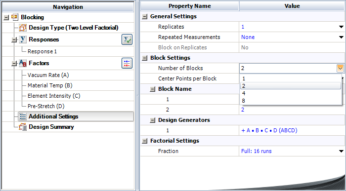
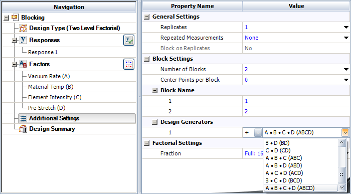

For the analysis of this design, the sum of squares for all effects are calculated assuming no blocking. Then, to account for blocking, the sum of squares corresponding to the [math]\displaystyle{ ABCD\,\! }[/math] interaction is considered as the sum of squares due to blocks and [math]\displaystyle{ ABCD\,\! }[/math]. In the DOE folio, this is done by displaying this sum of squares as the sum of squares due to the blocks. This is shown in the following figure where the sum of squares in question is obtained as 72.25 and is displayed against Block. The interaction ABCD, which is confounded with the blocks, is not displayed. Since the design is unreplicated, any of the methods to analyze unreplicated designs mentioned in Unreplicated [math]\displaystyle{ 2^k }[/math] designs have to be used to identify significant effects.
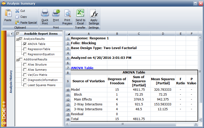
Unreplicated 2k Designs in 2p Blocks
A single replicate of the [math]\displaystyle{ {2}^{k}\,\! }[/math] design can be run in up to [math]\displaystyle{ {2}^{p}\,\! }[/math] blocks where [math]\displaystyle{ p\lt k\,\! }[/math]. The number of effects confounded with the blocks equals the degrees of freedom associated with the block effect.
If two blocks are used (the block effect has two levels), then one ([math]\displaystyle{ 2-1=1)\,\! }[/math] effect is confounded with the blocks. If four blocks are used, then three ([math]\displaystyle{ 4-1=3\,\! }[/math]) effects are confounded with the blocks and so on. For example an unreplicated [math]\displaystyle{ {2}^{4}\,\! }[/math] design may be confounded in [math]\displaystyle{ {2}^{2}\,\! }[/math] (four) blocks using two contrasts, [math]\displaystyle{ {{L}_{1}}\,\! }[/math] and [math]\displaystyle{ {{L}_{2}}\,\! }[/math]. Let [math]\displaystyle{ AC\,\! }[/math] and [math]\displaystyle{ BD\,\! }[/math] be the effects to be confounded with the blocks. Corresponding to these two effects, the contrasts are respectively:
- [math]\displaystyle{ \begin{align} & {{L}_{1}}= & {{q}_{1}}+{{q}_{3}} \\ & {{L}_{2}}= & {{q}_{2}}+{{q}_{4}} \end{align}\,\! }[/math]
Based on the values of [math]\displaystyle{ {{L}_{1}}\,\! }[/math] and [math]\displaystyle{ {{L}_{2}},\,\! }[/math] the treatments can be assigned to the four blocks as follows:
Since the block effect has three degrees of freedom, three effects are confounded with the block effect. In addition to [math]\displaystyle{ AC\,\! }[/math] and [math]\displaystyle{ BD\,\! }[/math], the third effect confounded with the block effect is their generalized interaction, [math]\displaystyle{ (AC)(BD)=ABCD\,\! }[/math].
In general, when an unreplicated [math]\displaystyle{ {2}^{k}\,\! }[/math] design is confounded in [math]\displaystyle{ {2}^{p}\,\! }[/math] blocks, [math]\displaystyle{ p\,\! }[/math] contrasts are needed ([math]\displaystyle{ {{L}_{1}},{{L}_{2}}...{{L}_{p}}\,\! }[/math]). [math]\displaystyle{ p\,\! }[/math] effects are selected to define these contrasts such that none of these effects are the generalized interaction of the others. The [math]\displaystyle{ {2}^{p}\,\! }[/math] blocks can then be assigned the treatments using the [math]\displaystyle{ p\,\! }[/math] contrasts. [math]\displaystyle{ {{2}^{p}}-(p+1)\,\! }[/math] effects, that are also confounded with the blocks, are then obtained as the generalized interaction of the [math]\displaystyle{ p\,\! }[/math] effects. In the statistical analysis of these designs, the sum of squares are computed as if no blocking were used. Then the block sum of squares is obtained by adding the sum of squares for all the effects confounded with the blocks.
Example: 2 Level Factorial Design with Four Blocks
This example illustrates how a DOE folio obtains the sum of squares when treatments for an unreplicated [math]\displaystyle{ {2}^{k}\,\! }[/math] design are allocated among four blocks. Consider again the unreplicated [math]\displaystyle{ {2}^{4}\,\! }[/math] design used to investigate the defects in automobile vinyl panels presented in Normal Probability Plot of Effects. Assume that the 16 treatments needed to complete the experiment were run by four operators. Therefore, there are four blocks. Assume that the treatments were allocated to the blocks using the generators mentioned in the previous section, i.e., treatments were allocated among the four operators by confounding the effects, [math]\displaystyle{ AC\,\! }[/math] and [math]\displaystyle{ BD,\,\! }[/math] with the blocks. These effects can be specified as Block Generators as shown in the following figure. (The generalized interaction of these two effects, interaction [math]\displaystyle{ ABCD\,\! }[/math], will also get confounded with the blocks.) The resulting design is shown in the second following figure and matches the allocation scheme obtained in the previous section.
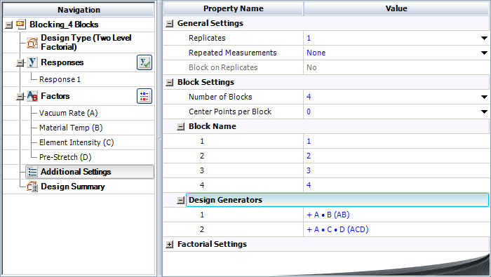
The sum of squares in this case can be obtained by calculating the sum of squares for each of the effects assuming there is no blocking. Once the individual sum of squares have been obtained, the block sum of squares can be calculated. The block sum of squares is the sum of the sum of squares of effects, [math]\displaystyle{ AC\,\! }[/math], [math]\displaystyle{ BD\,\! }[/math] and [math]\displaystyle{ ABCD\,\! }[/math], since these effects are confounded with the block effect. As shown in the second following figure, this sum of squares is 92.25 and is displayed against Block. The interactions [math]\displaystyle{ AC\,\! }[/math], [math]\displaystyle{ BD\,\! }[/math] and [math]\displaystyle{ ABCD\,\! }[/math], which are confounded with the blocks, are not displayed. Since the present design is unreplicated any of the methods to analyze unreplicated designs mentioned in Unreplicated [math]\displaystyle{ 2^k }[/math] designs have to be used to identify significant effects.
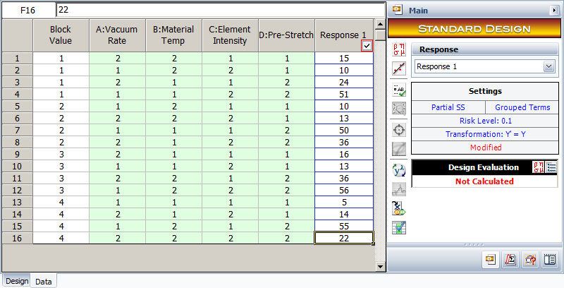
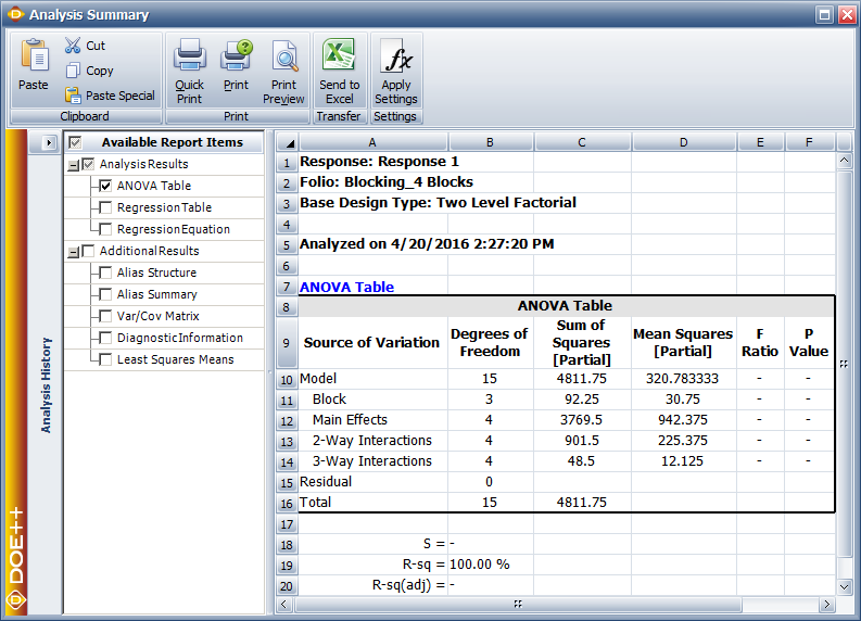
Variability Analysis
For replicated two level factorial experiments, the DOE folio provides the option of conducting variability analysis (using the Variability Analysis icon under the Data menu). The analysis is used to identify the treatment that results in the least amount of variation in the product or process being investigated. Variability analysis is conducted by treating the standard deviation of the response for each treatment of the experiment as an additional response. The standard deviation for a treatment is obtained by using the replicated response values at that treatment run. As an example, consider the [math]\displaystyle{ {2}^{3}\,\! }[/math] design shown in the following figure where each run is replicated four times. A variability analysis can be conducted for this design. The DOE folio calculates eight standard deviation values corresponding to each treatment of the design (see second following figure). Then, the design is analyzed as an unreplicated [math]\displaystyle{ {2}^{3}\,\! }[/math] design with the standard deviations (displayed as Y Standard Deviation. in second following figure) as the response. The normal probability plot of effects identifies [math]\displaystyle{ AC\,\! }[/math] as the effect that influences variability (see third figure following). Based on the effect coefficients obtained in the fourth figure following, the model for Y Std. is:
- [math]\displaystyle{ \begin{align} & \text{Y Std}\text{.}= & 0.6779+0.2491\cdot AC \\ & = & 0.6779+0.2491{{x}_{1}}{{x}_{3}} \end{align}\,\! }[/math]
Based on the model, the experimenter has two choices to minimize variability (by minimizing Y Std.). The first choice is that [math]\displaystyle{ {{x}_{1}}\,\! }[/math] should be [math]\displaystyle{ 1\,\! }[/math] (i.e., [math]\displaystyle{ A\,\! }[/math] should be set at the high level) and [math]\displaystyle{ {{x}_{3}}\,\! }[/math] should be [math]\displaystyle{ -1\,\! }[/math] (i.e., [math]\displaystyle{ C\,\! }[/math] should be set at the low level). The second choice is that [math]\displaystyle{ {{x}_{1}}\,\! }[/math] should be [math]\displaystyle{ -1\,\! }[/math] (i.e., [math]\displaystyle{ A\,\! }[/math] should be set at the low level) and [math]\displaystyle{ {{x}_{3}}\,\! }[/math] should be [math]\displaystyle{ -1\,\! }[/math] (i.e., [math]\displaystyle{ C\,\! }[/math] should be set at the high level). The experimenter can select the most feasible choice.
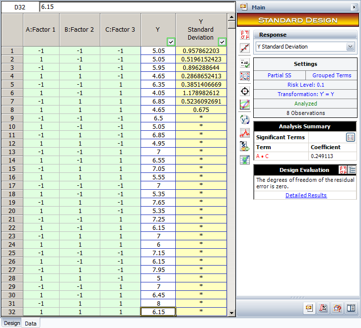
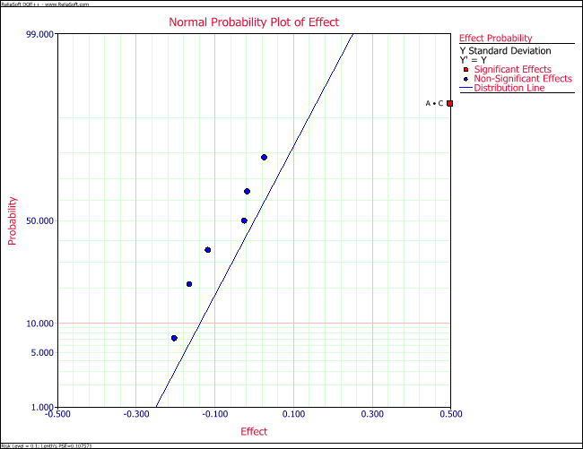
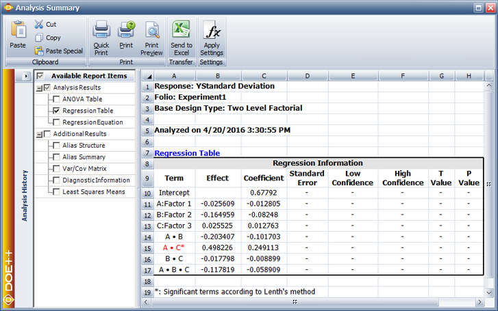

![The [math]\displaystyle{ 2^2\,\! }[/math] design. Figure (a) displays the experiment design, (b) displays the design matrix and (c) displays the geometric representation for the design. In Figure (b), the column names I, A, B and AB are used. Column I represents the intercept term. Columns A and B represent the respective factor settings. Column AB represents the interaction and is the product of columns A and B.](/images/c/c7/Doe7.2.png)
![The [math]\displaystyle{ 2^3\,\! }[/math] design. Figure (a) shows the experiment design and (b) shows the design matrix.](/images/d/dc/Doe7.3.png)
![Geometric representation of the [math]\displaystyle{ 2^3\,\! }[/math] design.](/images/3/3c/Doe7.4.png)

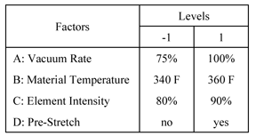
![[math]\displaystyle{ 2^2\,\! }[/math] design augmented by five center point runs.](/images/3/35/Doe7.17.png)
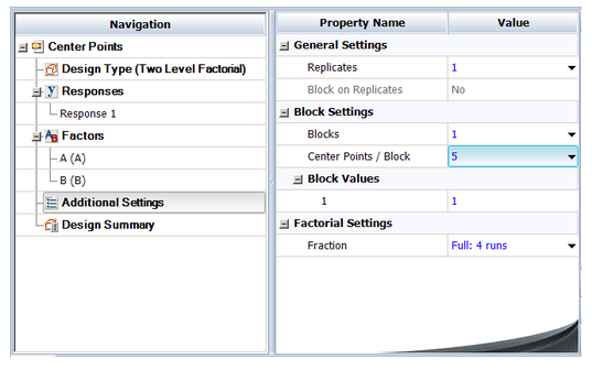
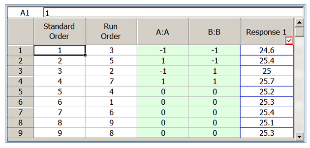
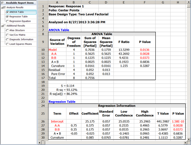
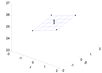
![Allocation of treatments to two blocks for the [math]\displaystyle{ 2^4 }[/math] design in the example by confounding interaction of [math]\displaystyle{ ABCD }[/math] with the blocks.](/images/d/d2/Doe7.22.png)
![A [math]\displaystyle{ 2^3\,\! }[/math] design with four replicated response values that can be used to conduct a variability analysis.](/images/4/45/Doe7.30.png)