Life Data Classification: Difference between revisions
Kate Racaza (talk | contribs) Undo revision 26937 by Kate Racaza (Talk) |
Lisa Hacker (talk | contribs) |
||
| (19 intermediate revisions by 6 users not shown) | |||
| Line 1: | Line 1: | ||
<noinclude>{{template:LDABOOK|5|Life Data Classifications}} | <noinclude>{{template:LDABOOK|5|Life Data Classifications}}</noinclude> | ||
<!-- NOTE: THE SECTIONS THAT ARE WITHIN THE "INCLUDEONLY" TAGS APPLY ONLY TO ALTA AND APPEAR ONLY IN THE PAGE: Accelerated_Life_Testing_and_ALTA. | |||
THE ENTIRE ARTICLE, THAT INCLUDES BOTH THE WEIBULL++ AND ALTA CONTENT, APPEAR IN THE PAGE: Types_of_Life_Data.--> | |||
Statistical models rely extensively on data to make predictions. In life data analysis, the models are the ''statistical distributions'' and the data are the ''life data'' or ''times-to-failure data'' of our product. <includeonly>In the case of accelerated life data analysis, the models are the ''life-stress relationships'' and the data are the ''times-to-failure data at a specific stress level''.</includeonly>The accuracy of any prediction is directly proportional to the quality, accuracy and completeness of the supplied data. Good data, along with the appropriate model choice, usually results in good predictions. Bad or insufficient data will almost always result in bad predictions. | |||
Statistical models rely extensively on data to make predictions. In | |||
In the analysis of life data, we want to use all available data sets, which sometimes are incomplete or include uncertainty as to when a failure occurred. Life data can therefore be separated into two types: ''complete data'' (all information is available) or ''censored data'' (some of the information is missing). Each type is explained next. | In the analysis of life data, we want to use all available data sets, which sometimes are incomplete or include uncertainty as to when a failure occurred. Life data can therefore be separated into two types: ''complete data'' (all information is available) or ''censored data'' (some of the information is missing). Each type is explained next. | ||
==Complete Data== | |||
Complete data means that the value of each sample unit is observed or known. For example, if we had to compute the average test score for a sample of ten students, complete data would consist of the known score for each student. Likewise in the case of life data analysis, our data set (if complete) would be composed of the times-to-failure of all units in our sample. For example, if we tested five units and they all failed (and their times-to-failure were recorded), we would then have complete information as to the time of each failure in the sample. | Complete data means that the value of each sample unit is observed or known. For example, if we had to compute the average test score for a sample of ten students, complete data would consist of the known score for each student. Likewise in the case of life data analysis, our data set (if complete) would be composed of the times-to-failure of all units in our sample. For example, if we tested five units and they all failed (and their times-to-failure were recorded), we would then have complete information as to the time of each failure in the sample. | ||
[[Image:complete data.png|center|400px|]] | [[Image:complete data.png|center|400px|]] | ||
==Censored Data == | |||
In many cases, all of the units in the sample may not have failed (i.e., the event of interest was not observed) or the exact times-to-failure of all the units are not known. This type of data is commonly called ''censored data''. There are three types of possible censoring schemes, right censored (also called suspended data), interval censored and left censored. | In many cases, all of the units in the sample may not have failed (i.e., the event of interest was not observed) or the exact times-to-failure of all the units are not known. This type of data is commonly called ''censored data''. There are three types of possible censoring schemes, right censored (also called suspended data), interval censored and left censored. | ||
===Right Censored (Suspension) Data=== | |||
The most common case of censoring is what is referred to as ''right censored data'', or ''suspended data''. In the case of life data, these data sets are composed of units that did not fail. For example, if we tested five units and only three had failed by the end of the test, we would have right censored data (or suspension data) for the two units that did not failed. The term ''right censored'' implies that the event of interest (i.e., the time-to-failure) is to the right of our data point. In other words, if the units were to keep on operating, the failure would occur at some time after our data point (or to the right on the time scale). | |||
The most common case of censoring is what is referred to as ''right censored data'', or ''suspended data''. In the case of life data, these data sets are composed of units that did not fail. For example, if we tested five units and only three had failed by the end of the test, we would have right censored data (or | |||
[[Image:right censoring.png|center|400px|Graphical representation of right censored data.]] | [[Image:right censoring.png|center|400px|Graphical representation of right censored data.]] | ||
===Interval Censored Data=== | |||
The second type of censoring is commonly called ''interval censored data''. Interval censored data reflects uncertainty as to the exact times the units failed within an interval. This type of data frequently comes from tests or situations where the objects of interest are not constantly monitored. For example, if we are running a test on five units and inspecting them every 100 hours, we only know that a unit failed or did not fail between inspections. Specifically, if we inspect a certain unit at 100 hours and find it operating, and then perform another inspection at 200 hours to find that the unit is no longer operating, then the only information we have is that the unit failed at some point in the interval between 100 and 200 hours. This type of censored data is also called ''inspection data'' by some authors. | The second type of censoring is commonly called ''interval censored data''. Interval censored data reflects uncertainty as to the exact times the units failed within an interval. This type of data frequently comes from tests or situations where the objects of interest are not constantly monitored. For example, if we are running a test on five units and inspecting them every 100 hours, we only know that a unit failed or did not fail between inspections. Specifically, if we inspect a certain unit at 100 hours and find it operating, and then perform another inspection at 200 hours to find that the unit is no longer operating, then the only information we have is that the unit failed at some point in the interval between 100 and 200 hours. This type of censored data is also called ''inspection data'' by some authors. | ||
| Line 32: | Line 26: | ||
It is generally recommended to avoid interval censored data because they are less informative compared to complete data. However, there are cases when interval data are unavoidable due to the nature of the product, the test and the test equipment. In those cases, caution must be taken to set the inspection intervals to be short enough to observe the spread of the failures. For example, if the inspection interval is too long, all the units in the test may fail within that interval, and thus no failure distribution could be obtained. | |||
The third type of censoring is similar to the interval censoring and is called ''left censored data''. In left censored data, a failure time is only known to be before a certain time. For instance, we may know that a certain unit failed sometime before 100 hours but not exactly when. In other words, it could have failed any time between 0 and 100 hours. This is identical to ''interval censored data''in which the starting time for the interval is zero. | |||
<includeonly>In the case of accelerated life tests, the data set affects the accuracy of the fitted life-stress relationship, and subsequently, the extrapolation to Use Stress conditions. In this case, inspection intervals should be chosen according to the expected acceleration factor at each stress level, and therefore these intervals will be of different lengths for each stress level. | |||
</includeonly>===Left Censored Data=== | |||
The third type of censoring is similar to the interval censoring and is called ''left censored data''. In left censored data, a failure time is only known to be before a certain time. For instance, we may know that a certain unit failed sometime before 100 hours but not exactly when. In other words, it could have failed any time between 0 and 100 hours. This is identical to ''interval censored data'' in which the starting time for the interval is zero. | |||
[[Image:left censoring.png|center|400px|]] | [[Image:left censoring.png|center|400px|]] | ||
===Grouped Data Analysis=== | |||
In the standard folio, data can be entered individually or in groups. Grouped data analysis is used for tests in which groups of units possess the same time-to-failure or in which groups of units were suspended at the same time. We highly recommend entering redundant data in groups. Grouped data speeds data entry by the user and significantly speeds up the calculations. | |||
==A Note about Complete and Suspension Data== | |||
Depending on the event that we want to measure, data type classification (i.e., complete or suspension) can be open to interpretation. For example, under certain circumstances, and depending on the question one wishes to answer, a specimen that has failed might be classified as a suspension for analysis purposes. To illustrate this, consider the following times-to-failure data for a product that can fail due to modes A, B and C: | |||
[[Image:time to failure chart.png|center|300px| ]] | |||
If the objective of the analysis is to determine the probability of failure of the product, regardless of the mode responsible for the failure, we would analyze the data with all data entries classified as failures (complete data). However, if the objective of the analysis is to determine the probability of failure of the product due to Mode A only, we would then choose to treat failures due to Modes B or C as suspension (right censored) data. Those data points would be treated as suspension data with respect to Mode A because the product operated until the recorded time without failure due to Mode A. | |||
==Fractional Failures== | |||
After the completion of a reliability test or after failures are observed in the field, a redesign can be implemented to improve a product’s reliability. After the redesign, and before new failure data become available, it is often times desirable to “adjust” the reliability that was calculated from the previous design and take “credit” for this theoretical improvement. This can be achieved with fractional failures. Using past experience to estimate the effectiveness of a corrective action or redesign, an analysis can take credit for this improvement by adjusting the failure count. Therefore, if a corrective action on a failure mode is believed to be 70% effective, then the failure count can be reduced from 1 to 0.3 to reflect the effectiveness of the corrective action. | |||
For example, consider the following data set. | |||
{| border="1" align="center" style="border-collapse: collapse;" cellpadding="5" cellspacing="5" | |||
|- align="center" | |||
!Number in State | |||
!State F or S | |||
!State End Time (Hr) | |||
|- align="center" | |||
|1 ||F || 105 | |||
|- align="center" | |||
|0.4 ||F || 168 | |||
|- align="center" | |||
|1 ||F || 220 | |||
|- align="center" | |||
|1 ||F || 290 | |||
|- align="center" | |||
|1 ||F || 410 | |||
|} | |||
In this case, a design change has been implemented for the failure mode that occurred at 168 hours and is assumed to be 60% effective. In the background, Weibull++ converts this data set to: | |||
{| border="1" align="center" style="border-collapse: collapse;" cellpadding="5" cellspacing="5" | |||
|- align="center" | |||
!Number in State | |||
!State F or S | |||
!State End Time (Hr) | |||
|- align="center" | |||
|1 ||F || 105 | |||
|- align="center" | |||
|0.4 ||F || 168 | |||
|- align="center" | |||
|0.6 ||S || 168 | |||
|- align="center" | |||
|1 ||F || 220 | |||
|- align="center" | |||
|1 ||F || 290 | |||
|- align="center" | |||
|1 ||F || 410 | |||
|} | |||
If [[Parameter Estimation|Rank Regression]] is used to estimate distribution parameters, the median ranks for the previous data set are calculated as follows: | |||
{| border="1" align="center" style="border-collapse: collapse;" cellpadding="5" cellspacing="5" | |||
|- align="center" | |||
!Number in State | |||
!State F or S | |||
!State End Time (Hr) | |||
!MON | |||
!Median Rank (%) | |||
|- align="center" | |||
|1 ||F || 105 || 1 ||12.945 | |||
|- align="center" | |||
|0.4 ||F || 168 || 1.4 | 20.267 | |||
|- align="center" | |||
|0.6 ||S || 168|| - || - | |||
|- align="center" | |||
|1 ||F || 220 || 2.55 || 41.616 | |||
|- align="center" | |||
|1 ||F || 290 || 3.7 || 63.039 | |||
|- align="center" | |||
|1 ||F || 410 || 4.85 || 84.325 | |||
|} | |||
Given this information, the standard Rank Regression procedure is then followed to estimate parameters. | |||
If [[Maximum Likelihood Estimation|Maximum Likelihood Estimation (MLE)]] is used to estimate distribution parameters, the grouped data likelihood function is used with the number in group being a non-integer value. | |||
===Example=== | |||
A component underwent a reliability test. 12 samples were run to failure. The following figure shows the failures and the analysis in a Weibull++ standard folio. | |||
[[Image:Fractional Failures 1.png|center|700px| ]] | |||
The analysts believe that the planned design improvements will yield 50% effectiveness. To estimate the reliability of the product based on the assumptions about the repair effectiveness, they enter the data in groups, counting a 0.5 failure for each group. The following figure shows the adjusted data set and the calculated parameters. | |||
[[Image:Fractional Failures 2.png|center|700px| ]] | |||
The following overlay plot of unreliability vs. time shows that by using fractional failures the estimated unreliability of the component has decreased, while the B10 life has increased from 2,566 hours to 3,564 hours. | |||
[[Image:Fractional Failures 4.png|center|650px| ]] | |||
Latest revision as of 00:54, 9 March 2023
Statistical models rely extensively on data to make predictions. In life data analysis, the models are the statistical distributions and the data are the life data or times-to-failure data of our product. The accuracy of any prediction is directly proportional to the quality, accuracy and completeness of the supplied data. Good data, along with the appropriate model choice, usually results in good predictions. Bad or insufficient data will almost always result in bad predictions.
In the analysis of life data, we want to use all available data sets, which sometimes are incomplete or include uncertainty as to when a failure occurred. Life data can therefore be separated into two types: complete data (all information is available) or censored data (some of the information is missing). Each type is explained next.
Complete Data
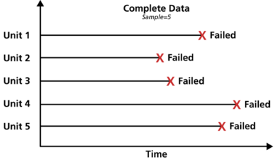
Complete data means that the value of each sample unit is observed or known. For example, if we had to compute the average test score for a sample of ten students, complete data would consist of the known score for each student. Likewise in the case of life data analysis, our data set (if complete) would be composed of the times-to-failure of all units in our sample. For example, if we tested five units and they all failed (and their times-to-failure were recorded), we would then have complete information as to the time of each failure in the sample.
Censored Data
In many cases, all of the units in the sample may not have failed (i.e., the event of interest was not observed) or the exact times-to-failure of all the units are not known. This type of data is commonly called censored data. There are three types of possible censoring schemes, right censored (also called suspended data), interval censored and left censored.
Right Censored (Suspension) Data
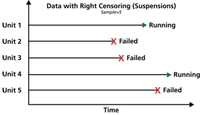
The most common case of censoring is what is referred to as right censored data, or suspended data. In the case of life data, these data sets are composed of units that did not fail. For example, if we tested five units and only three had failed by the end of the test, we would have right censored data (or suspension data) for the two units that did not failed. The term right censored implies that the event of interest (i.e., the time-to-failure) is to the right of our data point. In other words, if the units were to keep on operating, the failure would occur at some time after our data point (or to the right on the time scale).
Interval Censored Data
The second type of censoring is commonly called interval censored data. Interval censored data reflects uncertainty as to the exact times the units failed within an interval. This type of data frequently comes from tests or situations where the objects of interest are not constantly monitored. For example, if we are running a test on five units and inspecting them every 100 hours, we only know that a unit failed or did not fail between inspections. Specifically, if we inspect a certain unit at 100 hours and find it operating, and then perform another inspection at 200 hours to find that the unit is no longer operating, then the only information we have is that the unit failed at some point in the interval between 100 and 200 hours. This type of censored data is also called inspection data by some authors.
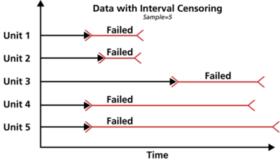
It is generally recommended to avoid interval censored data because they are less informative compared to complete data. However, there are cases when interval data are unavoidable due to the nature of the product, the test and the test equipment. In those cases, caution must be taken to set the inspection intervals to be short enough to observe the spread of the failures. For example, if the inspection interval is too long, all the units in the test may fail within that interval, and thus no failure distribution could be obtained.
Left Censored Data
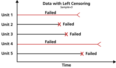
The third type of censoring is similar to the interval censoring and is called left censored data. In left censored data, a failure time is only known to be before a certain time. For instance, we may know that a certain unit failed sometime before 100 hours but not exactly when. In other words, it could have failed any time between 0 and 100 hours. This is identical to interval censored data in which the starting time for the interval is zero.
Grouped Data Analysis
In the standard folio, data can be entered individually or in groups. Grouped data analysis is used for tests in which groups of units possess the same time-to-failure or in which groups of units were suspended at the same time. We highly recommend entering redundant data in groups. Grouped data speeds data entry by the user and significantly speeds up the calculations.
A Note about Complete and Suspension Data
Depending on the event that we want to measure, data type classification (i.e., complete or suspension) can be open to interpretation. For example, under certain circumstances, and depending on the question one wishes to answer, a specimen that has failed might be classified as a suspension for analysis purposes. To illustrate this, consider the following times-to-failure data for a product that can fail due to modes A, B and C:
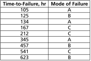
If the objective of the analysis is to determine the probability of failure of the product, regardless of the mode responsible for the failure, we would analyze the data with all data entries classified as failures (complete data). However, if the objective of the analysis is to determine the probability of failure of the product due to Mode A only, we would then choose to treat failures due to Modes B or C as suspension (right censored) data. Those data points would be treated as suspension data with respect to Mode A because the product operated until the recorded time without failure due to Mode A.
Fractional Failures
After the completion of a reliability test or after failures are observed in the field, a redesign can be implemented to improve a product’s reliability. After the redesign, and before new failure data become available, it is often times desirable to “adjust” the reliability that was calculated from the previous design and take “credit” for this theoretical improvement. This can be achieved with fractional failures. Using past experience to estimate the effectiveness of a corrective action or redesign, an analysis can take credit for this improvement by adjusting the failure count. Therefore, if a corrective action on a failure mode is believed to be 70% effective, then the failure count can be reduced from 1 to 0.3 to reflect the effectiveness of the corrective action.
For example, consider the following data set.
| Number in State | State F or S | State End Time (Hr) |
|---|---|---|
| 1 | F | 105 |
| 0.4 | F | 168 |
| 1 | F | 220 |
| 1 | F | 290 |
| 1 | F | 410 |
In this case, a design change has been implemented for the failure mode that occurred at 168 hours and is assumed to be 60% effective. In the background, Weibull++ converts this data set to:
| Number in State | State F or S | State End Time (Hr) |
|---|---|---|
| 1 | F | 105 |
| 0.4 | F | 168 |
| 0.6 | S | 168 |
| 1 | F | 220 |
| 1 | F | 290 |
| 1 | F | 410 |
If Rank Regression is used to estimate distribution parameters, the median ranks for the previous data set are calculated as follows:
| Number in State | State F or S | State End Time (Hr) | MON | Median Rank (%) |
|---|---|---|---|---|
| 1 | F | 105 | 1 | 12.945 |
| 0.4 | F | 168 | 20.267 | |
| 0.6 | S | 168 | - | - |
| 1 | F | 220 | 2.55 | 41.616 |
| 1 | F | 290 | 3.7 | 63.039 |
| 1 | F | 410 | 4.85 | 84.325 |
Given this information, the standard Rank Regression procedure is then followed to estimate parameters.
If Maximum Likelihood Estimation (MLE) is used to estimate distribution parameters, the grouped data likelihood function is used with the number in group being a non-integer value.
Example
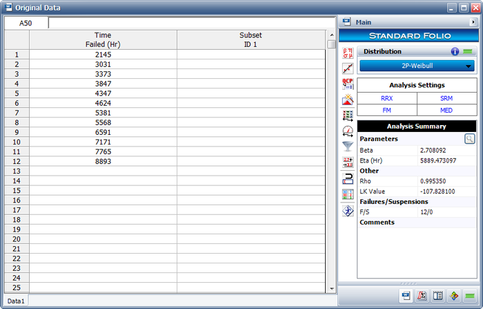
A component underwent a reliability test. 12 samples were run to failure. The following figure shows the failures and the analysis in a Weibull++ standard folio.
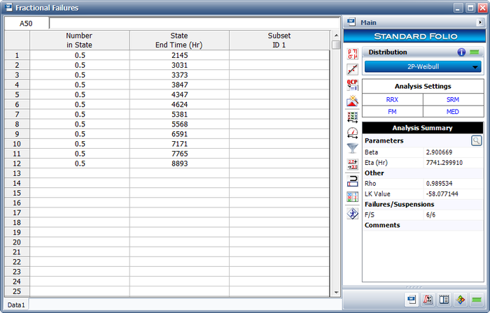
The analysts believe that the planned design improvements will yield 50% effectiveness. To estimate the reliability of the product based on the assumptions about the repair effectiveness, they enter the data in groups, counting a 0.5 failure for each group. The following figure shows the adjusted data set and the calculated parameters.
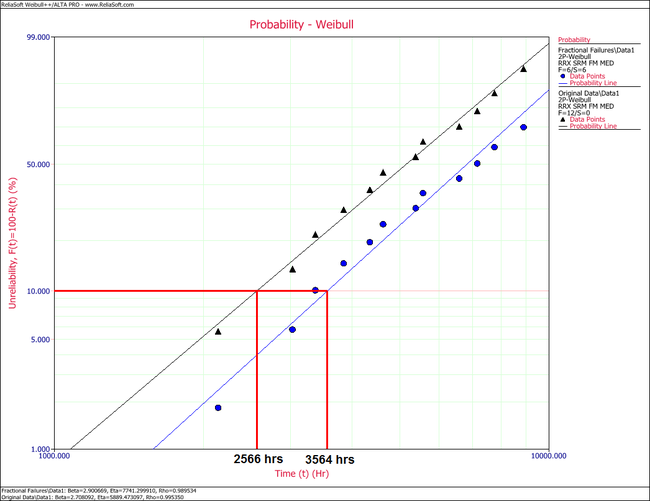
The following overlay plot of unreliability vs. time shows that by using fractional failures the estimated unreliability of the component has decreased, while the B10 life has increased from 2,566 hours to 3,564 hours.
