The Gamma Distribution: Difference between revisions
| (18 intermediate revisions by 3 users not shown) | |||
| Line 1: | Line 1: | ||
{{template:LDABOOK|13|The Gamma Distribution}} | {{template:LDABOOK|13|The Gamma Distribution}} | ||
The gamma distribution is a flexible life distribution model that may offer a good fit to some sets of failure data. It is not, however, widely used as a life distribution model for common failure mechanisms. The gamma distribution does arise naturally as the time-to-first-fail distribution for a system with standby exponentially distributed backups, and is also a good fit for the sum of independent exponential random variables. The gamma distribution is sometimes called the Erlang distribution, which is used frequently in queuing theory applications, as discussed in [[Appendix:_Life_Data_Analysis_References|[32]]]. | |||
The | ===The Gamma Probability Density Function=== | ||
The ''pdf'' of the gamma distribution is given by: | |||
::<math>f(t)=\frac{{{e}^{kz-{{e}^{z}}}}}{t\Gamma (k)}\,\!</math> | |||
::<math>f(t)=\frac{{{e}^{kz-{{e}^{z}}}}}{t\Gamma (k)}</math> | |||
where: | where: | ||
::<math>z=\ln (t)-\mu </math> | ::<math>\begin{align} | ||
z=\ln (t)-\mu | |||
\end{align}\,\!</math> | |||
and: | and: | ||
| Line 18: | Line 18: | ||
& {{e}^{\mu }}= \text{scale parameter} \\ | & {{e}^{\mu }}= \text{scale parameter} \\ | ||
& k= \text{shape parameter} | & k= \text{shape parameter} | ||
\end{align} | \end{align}\,\!</math> | ||
where <math>0<t<\infty \,\!</math>, <math>-\infty <\mu <\infty \,\!</math> and <math>k>0\,\!</math>. | |||
===The Gamma Reliability Function=== | ===The Gamma Reliability Function=== | ||
The reliability for a mission of time | The reliability for a mission of time <math>t\,\!</math> for the gamma distribution is: | ||
::<math>R=1-{{\Gamma }_{I}}(k;{{e}^{z}})</math> | ::<math>\begin{align} | ||
R=1-{{\Gamma }_{I}}(k;{{e}^{z}}) | |||
\end{align}\,\!</math> | |||
===The Gamma Mean, Median and Mode=== | ===The Gamma Mean, Median and Mode=== | ||
The gamma mean or MTTF is: | The gamma mean or MTTF is: | ||
::<math>\overline{T}=k{{e}^{\mu }}</math> | ::<math>\overline{T}=k{{e}^{\mu }}\,\!</math> | ||
The mode exists if | The mode exists if <math>k>1\,\!</math> and is given by: | ||
::<math>\tilde{T}=(k-1){{e}^{\mu }}</math> | ::<math>\tilde{T}=(k-1){{e}^{\mu }}\,\!</math> | ||
The median is: | The median is: | ||
::<math>\widehat{T}={{e}^{\mu +\ln (\Gamma _{I}^{-1}(0.5;k))}}</math> | ::<math>\widehat{T}={{e}^{\mu +\ln (\Gamma _{I}^{-1}(0.5;k))}}\,\!</math> | ||
===The Gamma Standard Deviation=== | ===The Gamma Standard Deviation=== | ||
The standard deviation for the gamma distribution is: | The standard deviation for the gamma distribution is: | ||
::<math>{{\sigma }_{T}}=\sqrt{k}{{e}^{\mu }}</math> | ::<math>{{\sigma }_{T}}=\sqrt{k}{{e}^{\mu }}\,\!</math> | ||
===The Gamma Reliable Life=== | ===The Gamma Reliable Life=== | ||
The gamma reliable life is: | The gamma reliable life is: | ||
::<math>{{T}_{R}}={{e}^{\mu +\ln (\Gamma _{1}^{-1}(1-R;k))}}</math> | ::<math>{{T}_{R}}={{e}^{\mu +\ln (\Gamma _{1}^{-1}(1-R;k))}}\,\!</math> | ||
===The Gamma Failure Rate Function=== | ===The Gamma Failure Rate Function=== | ||
The instantaneous gamma failure rate is given by: | The instantaneous gamma failure rate is given by: | ||
::<math>\lambda =\frac{{{e}^{kz-{{e}^{z}}}}}{t\Gamma (k)(1-{{\Gamma }_{I}}(k;{{e}^{z}}))}</math> | ::<math>\lambda =\frac{{{e}^{kz-{{e}^{z}}}}}{t\Gamma (k)(1-{{\Gamma }_{I}}(k;{{e}^{z}}))}\,\!</math> | ||
==Characteristics of the Gamma Distribution== | ==Characteristics of the Gamma Distribution== | ||
Some of the specific characteristics of the gamma distribution are the following: | Some of the specific characteristics of the gamma distribution are the following: | ||
For | For <math>k>1\,\!</math> : | ||
:• As | :• As <math>t\to 0,\infty\,\!</math>, <math>f(t)\to 0.\,\!</math> | ||
:• | :• <math>f(t)\,\!</math> increases from 0 to the mode value and decreases thereafter. | ||
:• If | :• If <math>k\le 2\,\!</math> then ''pdf'' has one inflection point at <math>t={{e}^{\mu }}\sqrt{k-1}(\,\!</math> <math>\sqrt{k-1}+1).\,\!</math> | ||
:• If | :• If <math>k>2\,\!</math> then ''pdf'' has two inflection points for <math>t={{e}^{\mu }}\sqrt{k-1}(\,\!</math> <math>\sqrt{k-1}\pm 1).\,\!</math> | ||
:• For a fixed | :• For a fixed <math>k\,\!</math>, as <math>\mu \,\!</math> increases, the ''pdf'' starts to look more like a straight angle. | ||
:• As | :• As <math>t\to \infty ,\lambda (t)\to \tfrac{1}{{{e}^{\mu }}}.\,\!</math> | ||
[[Image:BSpdf1.png|center| | [[Image:BSpdf1.png|center|400px| ]] | ||
For | For <math>k=1\,\!</math> : | ||
:• Gamma becomes the exponential distribution. | :• Gamma becomes the exponential distribution. | ||
:• As | :• As <math>t\to 0\,\!</math>, <math>f(T)\to \tfrac{1}{{{e}^{\mu }}}.\,\!</math> | ||
:• As | :• As <math>t\to \infty ,f(t)\to 0.\,\!</math> | ||
:• The | :• The ''pdf'' decreases monotonically and is convex. | ||
:• <math>\lambda (t)\equiv \tfrac{1}{{{e}^{\mu }}}</math> | :• <math>\lambda (t)\equiv \tfrac{1}{{{e}^{\mu }}}\,\!</math>. <math>\lambda (t)\,\!</math> is constant. | ||
:• The mode does not exist. | :• The mode does not exist. | ||
[[Image:BSpdf2.png|center| | [[Image:BSpdf2.png|center|400px| ]] | ||
For | For <math>0<k<1\,\!</math> : | ||
:• As | :• As <math>t\to 0\,\!</math>, <math>f(t)\to \infty .\,\!</math> | ||
:• As | :• As <math>t\to \infty ,f(t)\to 0.\,\!</math> | ||
:• As | :• As <math>t\to \infty ,\lambda (t)\to \tfrac{1}{{{e}^{\mu }}}.\,\!</math> | ||
:• The | :• The ''pdf'' decreases monotonically and is convex. | ||
:• As | :• As <math>\mu \,\!</math> increases, the ''pdf'' gets stretched out to the right and its height decreases, while maintaining its shape. | ||
:• As | :• As <math>\mu \,\!</math> decreases, the ''pdf'' shifts towards the left and its height increases. | ||
:• The mode does not exist. | :• The mode does not exist. | ||
[[Image:BSpdf3.png|center| | [[Image:BSpdf3.png|center|400px| ]] | ||
==Confidence Bounds== | ==Confidence Bounds== | ||
The only method available in Weibull++ for confidence bounds for the gamma distribution is the Fisher matrix, which is described next. The complete derivations were presented in detail (for a general function) in the [[Confidence Bounds]] chapter. | The only method available in Weibull++ for confidence bounds for the gamma distribution is the Fisher matrix, which is described next. The complete derivations were presented in detail (for a general function) in the [[Confidence Bounds]] chapter. | ||
===Bounds on the Parameters=== | ===Bounds on the Parameters=== | ||
The lower and upper bounds on the mean, | The lower and upper bounds on the mean, <math>\widehat{\mu }\,\!</math>, are estimated from: | ||
::<math>\begin{align} | ::<math>\begin{align} | ||
& {{\mu }_{U}}= & \widehat{\mu }+{{K}_{\alpha }}\sqrt{Var(\widehat{\mu })}\text{ (upper bound)} \\ | & {{\mu }_{U}}= & \widehat{\mu }+{{K}_{\alpha }}\sqrt{Var(\widehat{\mu })}\text{ (upper bound)} \\ | ||
& {{\mu }_{L}}= & \widehat{\mu }-{{K}_{\alpha }}\sqrt{Var(\widehat{\mu })}\text{ (lower bound)} | & {{\mu }_{L}}= & \widehat{\mu }-{{K}_{\alpha }}\sqrt{Var(\widehat{\mu })}\text{ (lower bound)} | ||
\end{align}</math> | \end{align}\,\!</math> | ||
Since the standard deviation, | Since the standard deviation, <math>\widehat{\sigma }\,\!</math>, must be positive, <math>\ln (\widehat{\sigma })\,\!</math> is treated as normally distributed and the bounds are estimated from: | ||
::<math>\begin{align} | ::<math>\begin{align} | ||
& {{k}_{U}}= & \widehat{k}\cdot {{e}^{\tfrac{{{K}_{\alpha }}\sqrt{Var(\widehat{k})}}{{\hat{k}}}}}\text{ (upper bound)} \\ | & {{k}_{U}}= & \widehat{k}\cdot {{e}^{\tfrac{{{K}_{\alpha }}\sqrt{Var(\widehat{k})}}{{\hat{k}}}}}\text{ (upper bound)} \\ | ||
& {{k}_{L}}= & \frac{\widehat{\sigma }}{{{e}^{\tfrac{{{K}_{\alpha }}\sqrt{Var(\widehat{k})}}{\widehat{k}}}}}\text{ (lower bound)} | & {{k}_{L}}= & \frac{\widehat{\sigma }}{{{e}^{\tfrac{{{K}_{\alpha }}\sqrt{Var(\widehat{k})}}{\widehat{k}}}}}\text{ (lower bound)} | ||
\end{align}</math> | \end{align}\,\!</math> | ||
where | where <math>{{K}_{\alpha }}\,\!</math> is defined by: | ||
::<math>\alpha =\frac{1}{\sqrt{2\pi }}\int_{{{K}_{\alpha }}}^{\infty }{{e}^{-\tfrac{{{t}^{2}}}{2}}}dt=1-\Phi ({{K}_{\alpha }})</math> | ::<math>\alpha =\frac{1}{\sqrt{2\pi }}\int_{{{K}_{\alpha }}}^{\infty }{{e}^{-\tfrac{{{t}^{2}}}{2}}}dt=1-\Phi ({{K}_{\alpha }})\,\!</math> | ||
If | If <math>\delta \,\!</math> is the confidence level, then <math>\alpha =\tfrac{1-\delta }{2}\,\!</math> for the two-sided bounds and <math>\alpha =1-\delta \,\!</math> for the one-sided bounds. | ||
The variances and covariances of | The variances and covariances of <math>\widehat{\mu }\,\!</math> and <math>\widehat{k}\,\!</math> are estimated from the Fisher matrix, as follows: | ||
::<math>\left( \begin{matrix} | ::<math>\left( \begin{matrix} | ||
| Line 129: | Line 124: | ||
{} & {} \\ | {} & {} \\ | ||
-\tfrac{{{\partial }^{2}}\Lambda }{\partial \mu \partial k} & -\tfrac{{{\partial }^{2}}\Lambda }{\partial {{k}^{2}}} \\ | -\tfrac{{{\partial }^{2}}\Lambda }{\partial \mu \partial k} & -\tfrac{{{\partial }^{2}}\Lambda }{\partial {{k}^{2}}} \\ | ||
\end{matrix} \right)_{\mu =\widehat{\mu },k=\widehat{k}}^{-1}</math> | \end{matrix} \right)_{\mu =\widehat{\mu },k=\widehat{k}}^{-1}\,\!</math> | ||
<math>\Lambda </math> | <math>\Lambda \,\!</math> is the log-likelihood function of the gamma distribution, described in [[Parameter Estimation]] and [[Appendix:_Log-Likelihood_Equations|Appendix D]] | ||
===Bounds on Reliability=== | ===Bounds on Reliability=== | ||
The reliability of the gamma distribution is: | The reliability of the gamma distribution is: | ||
::<math>\widehat{R}(t;\hat{\mu },\hat{k})=1-{{\Gamma }_{I}}(\widehat{k};{{e}^{\widehat{z}}})</math> | ::<math>\widehat{R}(t;\hat{\mu },\hat{k})=1-{{\Gamma }_{I}}(\widehat{k};{{e}^{\widehat{z}}})\,\!</math> | ||
where: | where: | ||
::<math>\widehat{z}=\ln (t)-\widehat{\mu }</math> | ::<math>\widehat{z}=\ln (t)-\widehat{\mu }\,\!</math> | ||
The upper and lower bounds on reliability are: | The upper and lower bounds on reliability are: | ||
::<math>{{R}_{U}}=\frac{\widehat{R}}{\widehat{R}+(1-\widehat{R})\exp (\tfrac{-{{K}_{\alpha }}\sqrt{Var(\widehat{R})\text{ }}}{\widehat{R}(1-\widehat{R})})}\text{ (upper bound)}</math> | ::<math>{{R}_{U}}=\frac{\widehat{R}}{\widehat{R}+(1-\widehat{R})\exp (\tfrac{-{{K}_{\alpha }}\sqrt{Var(\widehat{R})\text{ }}}{\widehat{R}(1-\widehat{R})})}\text{ (upper bound)}\,\!</math> | ||
::<math>{{R}_{L}}=\frac{\widehat{R}}{\widehat{R}+(1-\widehat{R})\exp (\tfrac{{{K}_{\alpha }}\sqrt{Var(\widehat{R})\text{ }}}{\widehat{R}(1-\widehat{R})})}\text{ (lower bound)}</math> | ::<math>{{R}_{L}}=\frac{\widehat{R}}{\widehat{R}+(1-\widehat{R})\exp (\tfrac{{{K}_{\alpha }}\sqrt{Var(\widehat{R})\text{ }}}{\widehat{R}(1-\widehat{R})})}\text{ (lower bound)}\,\!</math> | ||
where: | where: | ||
::<math>Var(\widehat{R})={{(\frac{\partial R}{\partial \mu })}^{2}}Var(\widehat{\mu })+2(\frac{\partial R}{\partial \mu })(\frac{\partial R}{\partial k})Cov(\widehat{\mu },\widehat{k})+{{(\frac{\partial z}{\partial k})}^{2}}Var(\widehat{k})</math> | ::<math>Var(\widehat{R})={{(\frac{\partial R}{\partial \mu })}^{2}}Var(\widehat{\mu })+2(\frac{\partial R}{\partial \mu })(\frac{\partial R}{\partial k})Cov(\widehat{\mu },\widehat{k})+{{(\frac{\partial z}{\partial k})}^{2}}Var(\widehat{k})\,\!</math> | ||
===Bounds on Time=== | ===Bounds on Time=== | ||
The bounds around time for a given gamma percentile (unreliability) are estimated by first solving the reliability equation with respect to time, as follows: | The bounds around time for a given gamma percentile (unreliability) are estimated by first solving the reliability equation with respect to time, as follows: | ||
::<math>\widehat{T}(\widehat{\mu },\widehat{\sigma })=\widehat{\mu }+\widehat{\sigma }z</math> | ::<math>\widehat{T}(\widehat{\mu },\widehat{\sigma })=\widehat{\mu }+\widehat{\sigma }z\,\!</math> | ||
where: | where: | ||
::<math>z=\ln (-\ln (R))</math> | ::<math>z=\ln (-\ln (R))\,\!</math> | ||
::<math>Var(\widehat{T})={{(\frac{\partial T}{\partial \mu })}^{2}}Var(\widehat{\mu })+2(\frac{\partial T}{\partial \mu })(\frac{\partial T}{\partial \sigma })Cov(\widehat{\mu },\widehat{\sigma })+{{(\frac{\partial T}{\partial \sigma })}^{2}}Var(\widehat{\sigma })</math> | ::<math>Var(\widehat{T})={{(\frac{\partial T}{\partial \mu })}^{2}}Var(\widehat{\mu })+2(\frac{\partial T}{\partial \mu })(\frac{\partial T}{\partial \sigma })Cov(\widehat{\mu },\widehat{\sigma })+{{(\frac{\partial T}{\partial \sigma })}^{2}}Var(\widehat{\sigma })\,\!</math> | ||
or: | or: | ||
::<math>Var(\widehat{T})=Var(\widehat{\mu })+2\widehat{z}Cov(\widehat{\mu },\widehat{\sigma })+{{\widehat{z}}^{2}}Var(\widehat{\sigma })</math> | ::<math>Var(\widehat{T})=Var(\widehat{\mu })+2\widehat{z}Cov(\widehat{\mu },\widehat{\sigma })+{{\widehat{z}}^{2}}Var(\widehat{\sigma })\,\!</math> | ||
The upper and lower bounds are then found by: | The upper and lower bounds are then found by: | ||
| Line 175: | Line 168: | ||
& {{T}_{U}}= & \hat{T}+{{K}_{\alpha }}\sqrt{Var(\hat{T})}\text{ (Upper bound)} \\ | & {{T}_{U}}= & \hat{T}+{{K}_{\alpha }}\sqrt{Var(\hat{T})}\text{ (Upper bound)} \\ | ||
& {{T}_{L}}= & \hat{T}-{{K}_{\alpha }}\sqrt{Var(\hat{T})}\text{ (Lower bound)} | & {{T}_{L}}= & \hat{T}-{{K}_{\alpha }}\sqrt{Var(\hat{T})}\text{ (Lower bound)} | ||
\end{align}</math> | \end{align}\,\!</math> | ||
==General Example== | ==General Example== | ||
{{ | {{:Gamma Distribution Example}} | ||
Latest revision as of 17:10, 23 December 2015
The gamma distribution is a flexible life distribution model that may offer a good fit to some sets of failure data. It is not, however, widely used as a life distribution model for common failure mechanisms. The gamma distribution does arise naturally as the time-to-first-fail distribution for a system with standby exponentially distributed backups, and is also a good fit for the sum of independent exponential random variables. The gamma distribution is sometimes called the Erlang distribution, which is used frequently in queuing theory applications, as discussed in [32].
The Gamma Probability Density Function
The pdf of the gamma distribution is given by:
- [math]\displaystyle{ f(t)=\frac{{{e}^{kz-{{e}^{z}}}}}{t\Gamma (k)}\,\! }[/math]
where:
- [math]\displaystyle{ \begin{align} z=\ln (t)-\mu \end{align}\,\! }[/math]
and:
- [math]\displaystyle{ \begin{align} & {{e}^{\mu }}= \text{scale parameter} \\ & k= \text{shape parameter} \end{align}\,\! }[/math]
where [math]\displaystyle{ 0\lt t\lt \infty \,\! }[/math], [math]\displaystyle{ -\infty \lt \mu \lt \infty \,\! }[/math] and [math]\displaystyle{ k\gt 0\,\! }[/math].
The Gamma Reliability Function
The reliability for a mission of time [math]\displaystyle{ t\,\! }[/math] for the gamma distribution is:
- [math]\displaystyle{ \begin{align} R=1-{{\Gamma }_{I}}(k;{{e}^{z}}) \end{align}\,\! }[/math]
The Gamma Mean, Median and Mode
The gamma mean or MTTF is:
- [math]\displaystyle{ \overline{T}=k{{e}^{\mu }}\,\! }[/math]
The mode exists if [math]\displaystyle{ k\gt 1\,\! }[/math] and is given by:
- [math]\displaystyle{ \tilde{T}=(k-1){{e}^{\mu }}\,\! }[/math]
The median is:
- [math]\displaystyle{ \widehat{T}={{e}^{\mu +\ln (\Gamma _{I}^{-1}(0.5;k))}}\,\! }[/math]
The Gamma Standard Deviation
The standard deviation for the gamma distribution is:
- [math]\displaystyle{ {{\sigma }_{T}}=\sqrt{k}{{e}^{\mu }}\,\! }[/math]
The Gamma Reliable Life
The gamma reliable life is:
- [math]\displaystyle{ {{T}_{R}}={{e}^{\mu +\ln (\Gamma _{1}^{-1}(1-R;k))}}\,\! }[/math]
The Gamma Failure Rate Function
The instantaneous gamma failure rate is given by:
- [math]\displaystyle{ \lambda =\frac{{{e}^{kz-{{e}^{z}}}}}{t\Gamma (k)(1-{{\Gamma }_{I}}(k;{{e}^{z}}))}\,\! }[/math]
Characteristics of the Gamma Distribution
Some of the specific characteristics of the gamma distribution are the following:
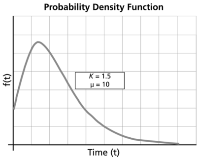
For [math]\displaystyle{ k\gt 1\,\! }[/math] :
- • As [math]\displaystyle{ t\to 0,\infty\,\! }[/math], [math]\displaystyle{ f(t)\to 0.\,\! }[/math]
- • [math]\displaystyle{ f(t)\,\! }[/math] increases from 0 to the mode value and decreases thereafter.
- • If [math]\displaystyle{ k\le 2\,\! }[/math] then pdf has one inflection point at [math]\displaystyle{ t={{e}^{\mu }}\sqrt{k-1}(\,\! }[/math] [math]\displaystyle{ \sqrt{k-1}+1).\,\! }[/math]
- • If [math]\displaystyle{ k\gt 2\,\! }[/math] then pdf has two inflection points for [math]\displaystyle{ t={{e}^{\mu }}\sqrt{k-1}(\,\! }[/math] [math]\displaystyle{ \sqrt{k-1}\pm 1).\,\! }[/math]
- • For a fixed [math]\displaystyle{ k\,\! }[/math], as [math]\displaystyle{ \mu \,\! }[/math] increases, the pdf starts to look more like a straight angle.
- • As [math]\displaystyle{ t\to \infty ,\lambda (t)\to \tfrac{1}{{{e}^{\mu }}}.\,\! }[/math]
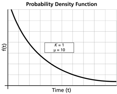
For [math]\displaystyle{ k=1\,\! }[/math] :
- • Gamma becomes the exponential distribution.
- • As [math]\displaystyle{ t\to 0\,\! }[/math], [math]\displaystyle{ f(T)\to \tfrac{1}{{{e}^{\mu }}}.\,\! }[/math]
- • As [math]\displaystyle{ t\to \infty ,f(t)\to 0.\,\! }[/math]
- • The pdf decreases monotonically and is convex.
- • [math]\displaystyle{ \lambda (t)\equiv \tfrac{1}{{{e}^{\mu }}}\,\! }[/math]. [math]\displaystyle{ \lambda (t)\,\! }[/math] is constant.
- • The mode does not exist.
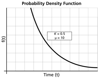
For [math]\displaystyle{ 0\lt k\lt 1\,\! }[/math] :
- • As [math]\displaystyle{ t\to 0\,\! }[/math], [math]\displaystyle{ f(t)\to \infty .\,\! }[/math]
- • As [math]\displaystyle{ t\to \infty ,f(t)\to 0.\,\! }[/math]
- • As [math]\displaystyle{ t\to \infty ,\lambda (t)\to \tfrac{1}{{{e}^{\mu }}}.\,\! }[/math]
- • The pdf decreases monotonically and is convex.
- • As [math]\displaystyle{ \mu \,\! }[/math] increases, the pdf gets stretched out to the right and its height decreases, while maintaining its shape.
- • As [math]\displaystyle{ \mu \,\! }[/math] decreases, the pdf shifts towards the left and its height increases.
- • The mode does not exist.
Confidence Bounds
The only method available in Weibull++ for confidence bounds for the gamma distribution is the Fisher matrix, which is described next. The complete derivations were presented in detail (for a general function) in the Confidence Bounds chapter.
Bounds on the Parameters
The lower and upper bounds on the mean, [math]\displaystyle{ \widehat{\mu }\,\! }[/math], are estimated from:
- [math]\displaystyle{ \begin{align} & {{\mu }_{U}}= & \widehat{\mu }+{{K}_{\alpha }}\sqrt{Var(\widehat{\mu })}\text{ (upper bound)} \\ & {{\mu }_{L}}= & \widehat{\mu }-{{K}_{\alpha }}\sqrt{Var(\widehat{\mu })}\text{ (lower bound)} \end{align}\,\! }[/math]
Since the standard deviation, [math]\displaystyle{ \widehat{\sigma }\,\! }[/math], must be positive, [math]\displaystyle{ \ln (\widehat{\sigma })\,\! }[/math] is treated as normally distributed and the bounds are estimated from:
- [math]\displaystyle{ \begin{align} & {{k}_{U}}= & \widehat{k}\cdot {{e}^{\tfrac{{{K}_{\alpha }}\sqrt{Var(\widehat{k})}}{{\hat{k}}}}}\text{ (upper bound)} \\ & {{k}_{L}}= & \frac{\widehat{\sigma }}{{{e}^{\tfrac{{{K}_{\alpha }}\sqrt{Var(\widehat{k})}}{\widehat{k}}}}}\text{ (lower bound)} \end{align}\,\! }[/math]
where [math]\displaystyle{ {{K}_{\alpha }}\,\! }[/math] is defined by:
- [math]\displaystyle{ \alpha =\frac{1}{\sqrt{2\pi }}\int_{{{K}_{\alpha }}}^{\infty }{{e}^{-\tfrac{{{t}^{2}}}{2}}}dt=1-\Phi ({{K}_{\alpha }})\,\! }[/math]
If [math]\displaystyle{ \delta \,\! }[/math] is the confidence level, then [math]\displaystyle{ \alpha =\tfrac{1-\delta }{2}\,\! }[/math] for the two-sided bounds and [math]\displaystyle{ \alpha =1-\delta \,\! }[/math] for the one-sided bounds.
The variances and covariances of [math]\displaystyle{ \widehat{\mu }\,\! }[/math] and [math]\displaystyle{ \widehat{k}\,\! }[/math] are estimated from the Fisher matrix, as follows:
- [math]\displaystyle{ \left( \begin{matrix} \widehat{Var}\left( \widehat{\mu } \right) & \widehat{Cov}\left( \widehat{\mu },\widehat{k} \right) \\ \widehat{Cov}\left( \widehat{\mu },\widehat{k} \right) & \widehat{Var}\left( \widehat{k} \right) \\ \end{matrix} \right)=\left( \begin{matrix} -\tfrac{{{\partial }^{2}}\Lambda }{\partial {{\mu }^{2}}} & -\tfrac{{{\partial }^{2}}\Lambda }{\partial \mu \partial k} \\ {} & {} \\ -\tfrac{{{\partial }^{2}}\Lambda }{\partial \mu \partial k} & -\tfrac{{{\partial }^{2}}\Lambda }{\partial {{k}^{2}}} \\ \end{matrix} \right)_{\mu =\widehat{\mu },k=\widehat{k}}^{-1}\,\! }[/math]
[math]\displaystyle{ \Lambda \,\! }[/math] is the log-likelihood function of the gamma distribution, described in Parameter Estimation and Appendix D
Bounds on Reliability
The reliability of the gamma distribution is:
- [math]\displaystyle{ \widehat{R}(t;\hat{\mu },\hat{k})=1-{{\Gamma }_{I}}(\widehat{k};{{e}^{\widehat{z}}})\,\! }[/math]
where:
- [math]\displaystyle{ \widehat{z}=\ln (t)-\widehat{\mu }\,\! }[/math]
The upper and lower bounds on reliability are:
- [math]\displaystyle{ {{R}_{U}}=\frac{\widehat{R}}{\widehat{R}+(1-\widehat{R})\exp (\tfrac{-{{K}_{\alpha }}\sqrt{Var(\widehat{R})\text{ }}}{\widehat{R}(1-\widehat{R})})}\text{ (upper bound)}\,\! }[/math]
- [math]\displaystyle{ {{R}_{L}}=\frac{\widehat{R}}{\widehat{R}+(1-\widehat{R})\exp (\tfrac{{{K}_{\alpha }}\sqrt{Var(\widehat{R})\text{ }}}{\widehat{R}(1-\widehat{R})})}\text{ (lower bound)}\,\! }[/math]
where:
- [math]\displaystyle{ Var(\widehat{R})={{(\frac{\partial R}{\partial \mu })}^{2}}Var(\widehat{\mu })+2(\frac{\partial R}{\partial \mu })(\frac{\partial R}{\partial k})Cov(\widehat{\mu },\widehat{k})+{{(\frac{\partial z}{\partial k})}^{2}}Var(\widehat{k})\,\! }[/math]
Bounds on Time
The bounds around time for a given gamma percentile (unreliability) are estimated by first solving the reliability equation with respect to time, as follows:
- [math]\displaystyle{ \widehat{T}(\widehat{\mu },\widehat{\sigma })=\widehat{\mu }+\widehat{\sigma }z\,\! }[/math]
where:
- [math]\displaystyle{ z=\ln (-\ln (R))\,\! }[/math]
- [math]\displaystyle{ Var(\widehat{T})={{(\frac{\partial T}{\partial \mu })}^{2}}Var(\widehat{\mu })+2(\frac{\partial T}{\partial \mu })(\frac{\partial T}{\partial \sigma })Cov(\widehat{\mu },\widehat{\sigma })+{{(\frac{\partial T}{\partial \sigma })}^{2}}Var(\widehat{\sigma })\,\! }[/math]
or:
- [math]\displaystyle{ Var(\widehat{T})=Var(\widehat{\mu })+2\widehat{z}Cov(\widehat{\mu },\widehat{\sigma })+{{\widehat{z}}^{2}}Var(\widehat{\sigma })\,\! }[/math]
The upper and lower bounds are then found by:
- [math]\displaystyle{ \begin{align} & {{T}_{U}}= & \hat{T}+{{K}_{\alpha }}\sqrt{Var(\hat{T})}\text{ (Upper bound)} \\ & {{T}_{L}}= & \hat{T}-{{K}_{\alpha }}\sqrt{Var(\hat{T})}\text{ (Lower bound)} \end{align}\,\! }[/math]
General Example
24 units were reliability tested, and the following life test data were obtained:
| 61 | 50 | 67 | 49 | 53 | 62 |
| 53 | 61 | 43 | 65 | 53 | 56 |
| 62 | 56 | 58 | 55 | 58 | 48 |
| 66 | 44 | 48 | 58 | 43 | 40 |
Fitting the gamma distribution to this data, using maximum likelihood as the analysis method, gives the following parameters:
- [math]\displaystyle{ \begin{align} & \hat{\mu }= 7.72E-02 \\ & \hat{k}= 50.4908 \end{align}\,\! }[/math]
Using rank regression on [math]\displaystyle{ X,\,\! }[/math] the estimated parameters are:
- [math]\displaystyle{ \begin{align} & \hat{\mu }= 0.2915 \\ & \hat{k}= 41.1726 \end{align}\,\! }[/math]
Using rank regression on [math]\displaystyle{ Y,\,\! }[/math] the estimated parameters are:
- [math]\displaystyle{ \begin{align} & \hat{\mu }= 0.2915 \\ & \hat{k}= 41.1726 \end{align}\,\! }[/math]


