Cumulative Damage Model for Step Stress Profiles: Difference between revisions
Jump to navigation
Jump to search
Kate Racaza (talk | contribs) No edit summary |
Kate Racaza (talk | contribs) No edit summary |
||
| (4 intermediate revisions by the same user not shown) | |||
| Line 1: | Line 1: | ||
{{Reference Example|{{Banner ALTA Reference Examples}}}} | {{Reference Example|{{Banner ALTA Reference Examples}}}} | ||
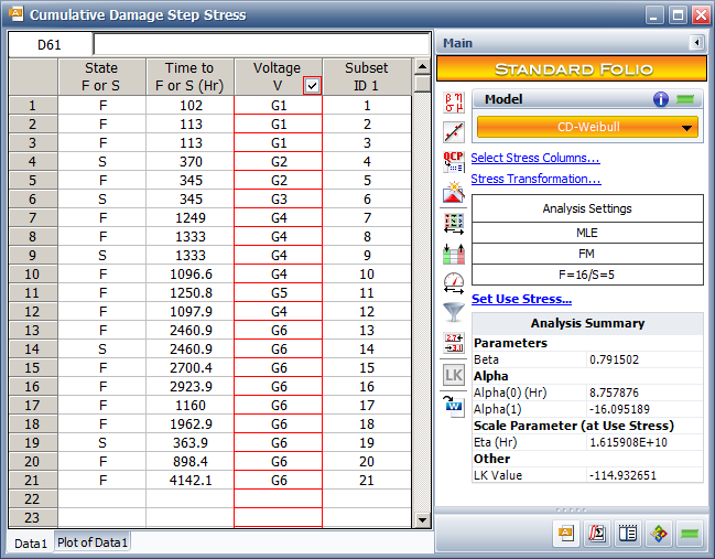
This example | This example validates the results for a cumulative damage model for a step stress test in an ALTA standard folio. | ||
| Line 11: | Line 11: | ||
{{Reference_Example_Heading2}} | {{Reference_Example_Heading2}} | ||
A step-stress test is conducted for one type of cable insulation to estimate the insulation life at a constant design stress of 400 volts/mil. The test cables are of different thickness, in | A step-stress test is conducted for one type of cable insulation to estimate the insulation life at a constant design stress of 400 volts/mil. The test cables are of different thickness, in units of mils (0.001 inch). The stress is the applied step voltage divided by the thickness. | ||
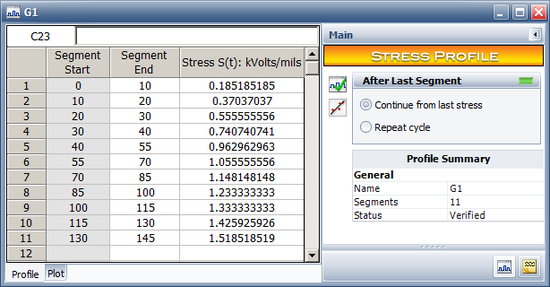
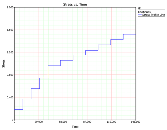
A total of 6 step-stress profiles are used. These stress profiles are calculated based on the applied voltage (Kilovolts) and the insulation thickness given on page 495 and Table 2.1. For all the stress profiles, the holding time for the first 4 steps is 10 mins. From step 5 onwards, a different a holding time is applied at each step for each of the stress profiles. These profiles are given in the following tables. | A total of 6 step-stress profiles are used. These stress profiles are calculated based on the applied voltage (Kilovolts) and the insulation thickness given on page 495 and Table 2.1. For all the stress profiles, the holding time for the first 4 steps is 10 mins. From step 5 onwards, a different a holding time is applied at each step for each of the stress profiles. These profiles are given in the following tables. | ||
| Line 257: | Line 257: | ||
{{Reference_Example_Heading3}} | {{Reference_Example_Heading3}} | ||
The power law life stress relationship and the Weibull distribution | The power law life stress relationship and the Weibull distribution are used to analyze the data. At a constant stress ''V'', the <math>\eta\,\!</math> is: | ||
::<math>\eta(V) = \left(\frac{V_{0}}{V} \right)^p\,\!</math> | ::<math>\eta(V) = \left(\frac{V_{0}}{V} \right)^p\,\!</math> | ||
where <math>V_{0}\,\!</math> and <math>p\,\!</math> are the model parameters used in the book. | where <math>V_{0}\,\!</math> and <math>p\,\!</math> are the model parameters used in the book. The above equation can be rewritten as: | ||
The above equation can be rewritten as: | |||
::<math>\eta(V) = e^{\alpha_{0}+\alpha_{1}ln(V)}\,\!</math> | ::<math>\eta(V) = e^{\alpha_{0}+\alpha_{1}ln(V)}\,\!</math> | ||
where <math>\alpha_{0} = | where <math>\alpha_{0} = p \cdot ln(V_{0})\,\!</math> and <math>\alpha_{1} = -p\,\!</math> | ||
| Line 325: | Line 322: | ||
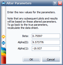
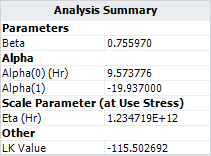
Using the parameters values originally calculated in ALTA: | Using the parameters values originally calculated in ALTA: | ||
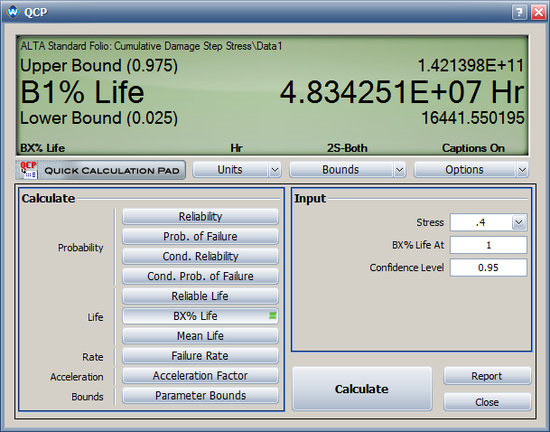
* The 1% percentile point (B1 life) at 0.4 Kvolts/mil is 4.8342 X 10<sup>7</sup> hours, as shown next. | * The 1% percentile point (B1 life) at 0.4 Kvolts/mil is 4.8342 X 10<sup>7</sup> hours, as shown next. The value given in the book is 2.81 X 10<sup>9</sup>. The results are different because of the differences in the values of the parameters of the model. | ||
[[Image: Step Stress qcp.png|center|550px]] | [[Image: Step Stress qcp.png|center|550px]] | ||
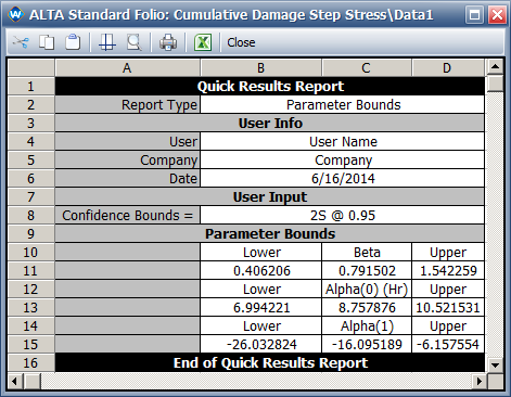
* The 2-sided 95% confidence intervals for model parameters are shown next. | * The 2-sided 95% confidence intervals for the model parameters are shown next. These results are also different from the results in the book due to the estimated parameter values. | ||
[[Image: Step Stress bounds.png|center]] | [[Image: Step Stress bounds.png|center]] | ||
| Line 341: | Line 338: | ||
Define the stress value at step ''i'' as <math>S_{i}\,\!</math>. If the test unit stayed in this stress level for a time period of <math>\Delta t_{i}\,\!</math>, then the cumulative damage at this step will be <math>\frac{1}{\eta(S_{i})}\times \Delta t_{i}\,\!</math> and | Define the stress value at step ''i'' as <math>S_{i}\,\!</math>. If the test unit stayed in this stress level for a time period of <math>\Delta t_{i}\,\!</math>, then the cumulative damage at this step will be <math>\frac{1}{\eta(S_{i})}\times \Delta t_{i}\,\!</math> and | ||
::<math>A_{i} = \frac{1}{\eta(S_{i})} \times \Delta t_{i} = e^{-(\alpha_{0}+\alpha_{1}ln(S_{ | ::<math>A_{i} = \frac{1}{\eta(S_{i})} \times \Delta t_{i} = e^{-(\alpha_{0}+\alpha_{1}ln(S_{i}))} \times \Delta t_{i}\,\!</math> | ||
For example, for the first failure, the failure occurred at 102, which is at the 9th step of profile G1. The test unit accumulates damage from each step stress it experienced before it fails. The first step stress value is 0.185185 which is the voltage divided by the thickness (5 Kvolts/27 mils). The length of the first step is 10 mins. Therefore, the damage at the 1st step segment is: | For example, for the first failure, the failure occurred at 102, which is at the 9th step of profile G1. The test unit accumulates damage from each step stress it experienced before it fails. The first step stress value is 0.185185, which is the voltage divided by the thickness (5 Kvolts/27 mils). The length of the first step is 10 mins. Therefore, the damage at the 1st step segment is: | ||
::<math>A_{1} = e^{-(\alpha_{0}+\alpha_{1}ln(S_{1}))} \times \Delta t_{i} = e^{-(8.757876+16.095189 \times 1.6864)}\times 10 = 2.56 \times 10^{-15}\,\!</math> | ::<math>A_{1} = e^{-(\alpha_{0}+\alpha_{1}ln(S_{1}))} \times \Delta t_{i} = e^{-(8.757876+16.095189 \times 1.6864)}\times 10 = 2.56 \times 10^{-15}\,\!</math> | ||
We can use this method to calculate the damage at each stress segment. The total damage will be the sum of the damage at each segment. For the first failure at time 102 under stress profile G1, the damage at each stress segment is calculated as given below. | We can use this method to calculate the damage at each stress segment. The total damage will be the sum of the damage at each segment. For the first failure at time 102 under stress profile G1, the damage at each stress segment is calculated, as given below. | ||
{| {{table}} | {| {{table}} | ||
| Line 372: | Line 369: | ||
| 9||100||102||36||27||1.333333||0.287682072||0.031977014 | | 9||100||102||36||27||1.333333||0.287682072||0.031977014 | ||
|- | |- | ||
| | |colspan="7" style="text-align:right;"|'''A ='''||0.132138165 | ||
|- | |- | ||
|} | |} | ||
The total | The total cumulative damage at a failure time of 102 is '''A''' in the above table. | ||
Since the reliability function is: | Since the reliability function is: | ||
::<math>R(t) = e^{-\left[\int^{t}_{0}e^{-(\alpha_{0}+\alpha_{1}ln(S(x)))} dx \right]^{\beta}} = e^{-A^{\beta}}\,\!</math> | |||
The probability density function (pdf) at time ''t'' is: | |||
::<math>\begin{align} | |||
f(t) =& R(t) \cdot \beta \cdot \left[\int^{t}_{0}e^{-(\alpha_{0}+\alpha_{1}ln(S(x)))} dx \right]^{\beta-1}\cdot e^{-(\alpha_{0}+\alpha_{1}ln(S(t)))} \\ | |||
=& e^{-A^{\beta}}\cdot \beta \cdot A^{\beta-1}\cdot e^{-(\alpha_{0}+\alpha_{1}ln(S(t)))} \\ | |||
\end{align}\,\!</math> | |||
If an observation is a failure, then the pdf will be used to calculate its log likelihood value. If an observation is a suspension, then the reliability will be used to calculate its log likelihood value. | |||
Since the 1st observation is a failure, the pdf is used. Using the model parameters and the cumulative damage A, the value of the pdf is: | |||
::<math> \begin{align} | |||
f(t) =& e^{-A^{\beta}} \cdot \beta \cdot A^{\beta - 1} \cdot e^{-(\alpha_{0}+\alpha_{1}ln(S(t)))} \\ | |||
=& e^{-0.13214^{0.7906}} \times 0.7906 \times 0.13214^{0.7906-1} \times e^{-(8.7685 - 16.103 \times 0.2877)} \\ | |||
=& 0.016 | |||
\end{align}\,\!</math> | |||
Take the logarithm of the above value and we get the log likelihood value for the first observation as <math>log(0.016) = -4.1489\,\!</math>. | |||
Repeating the above procedure, we can get the log likelihood value for each observation, as given in the following table. | |||
{| {{table}} | |||
! Status F/S||Time To F/S||Profile||Log likelihood Value | |||
|- | |||
| F||102||G1||-4.148929577 | |||
|- | |||
| F||113||G1||-4.518387096 | |||
|- | |||
| F||113||G1||-4.518387096 | |||
|- | |||
| S||370||G2||-0.72559186 | |||
|- | |||
| F||345||G2||-4.983506849 | |||
|- | |||
| S||345||G3||-0.910644661 | |||
|- | |||
| F||1249||G4||-6.199936981 | |||
|- | |||
| F||1333||G4||-7.129057207 | |||
|- | |||
| S||1333||G4||-2.451259934 | |||
|- | |||
| F||1096.6||G4||-6.518744419 | |||
|- | |||
| F||1250.8||G5||-6.075214111 | |||
|- | |||
| F||1097.9||G4||-6.523803805 | |||
|- | |||
| F||2460.9||G6||-8.444820079 | |||
|- | |||
| S||2460.9||G6||-0.29378846 | |||
|- | |||
| F||2700.4||G6||-8.566484581 | |||
|- | |||
| F||2923.9||G6||-7.469922325 | |||
|- | |||
| F||1160||G6||-9.119207934 | |||
|- | |||
| F||1962.9||G6||-8.086491838 | |||
|- | |||
| S||363.9||G6||-0.015237126 | |||
|- | |||
| F||898.4||G6||-10.4367511 | |||
|- | |||
| F||4142.1||G6||-7.897236924 | |||
|- | |||
|colspan = "3" style="text-align: right;"|'''Total'''||-115.033404 | |||
|- | |||
|} | |||
The log likelihood value calculated by hand in Microsoft Excel is -115.0334, as given in the above table. It matches the value in ALTA. The slight difference is caused by the precision error. Therefore, the log likelihood value calculated in ALTA is correct. | |||
In fact, the optimization tool in Excel can also be used to find the ML solutions. Using the “Solver Add-in” program in Excel and the “GRG” nonlinear optimization, we get the same results in Excel as in ALTA. | |||
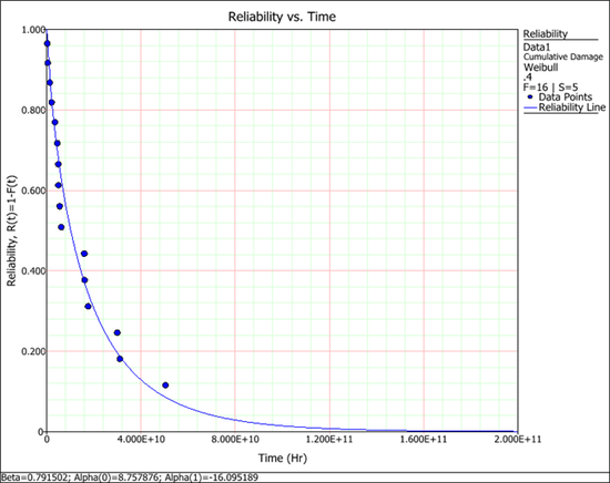
The following reliability plot shows that the predicted values (the line) by the model can match the observed values (the points) very well. | |||
[[Image:Step Stress_plot.png|center|550 px]] | |||
Latest revision as of 18:22, 28 September 2015
New format available! This reference is now available in a new format that offers faster page load, improved display for calculations and images and more targeted search.
As of January 2024, this Reliawiki page will not continue to be updated. Please update all links and bookmarks to the latest references at ALTA examples and ALTA reference examples.

