Arrhenius-Lognormal Model for Interval Data: Difference between revisions

From ReliaWiki
Jump to navigation Jump to search
No edit summary
No edit summary
 
(3 intermediate revisions by the same user not shown)
Line 1: Line 1:
{{Reference Example|ALTA_Reference_Examples_Banner.png|ALTA_Reference_Examples}}
{{Reference Example|{{Banner ALTA Reference Examples}}}}


This example compares the results for the Arrhenius-Lognormal model with interval data.
This example validates the results for the Arrhenius-lognormal model with interval data in ALTA standard folios.


Line 11: Line 11:
{{Reference_Example_Heading2}}


The data set for a new-technology IC Device is given below.
The data set for a new-technology IC device is given below.


{| {{table}}
{| {{table}}
Line 53: Line 53:


The above equation is the general log-linear model in ALTA. In ALTA, the coefficients are denoted by <math>\alpha_{i}\,\!</math>. We can see <math>\beta_{0} = \alpha_{0}\,\!</math> and <math>\beta_{1} = \frac{\alpha_{1}}{11605}\,\!</math>.
The above equation is the general log-linear model in ALTA. In ALTA, the coefficients are denoted by <math>\alpha_{i}\,\!</math>. We can see that <math>\beta_{0} = \alpha_{0}\,\!</math> and <math>\beta_{1} = \frac{\alpha_{1}}{11605}\,\!</math>.


In fact, the above model can also be expressed using the traditional Arrhenius model:
Line 62: Line 62:
In the book, the following results are provided:


* ML estimations for the model parameters are: <math>\sigma\,\!</math> = 0.52, <math>\beta_{0}\,\!</math> = -10.2, <math>\beta_{1}\,\!</math> = 0.83, (<math>\alpha_{1}\,\!</math> = <math>\beta_{1}\times  \,\!</math> 11605 = 9632.15).  
* The ML estimations for the model parameters are: <math>\sigma\,\!</math> = 0.52, <math>\beta_{0}\,\!</math> = -10.2, <math>\beta_{1}\,\!</math> = 0.83, (<math>\alpha_{1}\,\!</math> = <math>\beta_{1}\times  \,\!</math> 11605 = 9632.15).  
* The standard deviation of each parameter: <math>std(\sigma)\,\!</math>  = 0.06, &nbsp; <math>std(\beta_{0})\,\!</math>  = 1.5, &nbsp;<math>std(\beta_{1})\,\!</math>  = 0.07. Therefore, their variances are: <math>Var(\sigma)\,\!</math>  = 0.0036, &nbsp;<math>Var(\beta_{0})\,\!</math>  = 2.25, &nbsp;<math>Var(\beta_{1})\,\!</math>  = 0.0049. In terms of <math>\alpha_{1}\,\!</math> , the variance is <math>Var(\alpha_{1})\,\!</math>  = 11605<sup>2</sup> &nbsp;and&nbsp; <math>Var(\beta_{1})\,\!</math>  = 659912.5.
* The 95% two-sided confidence bounds are: for <math>\sigma\,\!</math> it is [0.42, 0.64]; for <math>\beta_{0}\,\!</math>  it is [-13.2, -7.2]; for <math>\beta_{1}\,\!</math> it is [0.68, 0.97]. In terms of <math>\alpha_{1}\,\!</math>, the bounds are [7891.14, 11256.85].  
Line 76: Line 76:


The picture above also shows the standard deviations of the parameters. These are: <math>std(\sigma)\,\!</math>  = 0.06, &nbsp; <math>std(\beta_{0})\,\!</math>  = 1.5, &nbsp;<math>std(\beta_{1})\,\!</math>  = 0.07. Therefore, their variances are: <math>Var(\sigma)\,\!</math>  = 0.0036, &nbsp;<math>Var(\beta_{0})\,\!</math>  = 2.25, &nbsp;<math>Var(\beta_{1})\,\!</math>  = 0.0049. In terms of <math>\alpha_{1}\,\!</math> , the variance is <math>Var(\alpha_{1})\,\!</math>  = 11605<sup>2</sup> &nbsp;and&nbsp; <math>Var(\beta_{1})\,\!</math>  = 659912.5.
The picture above also shows variance of each parameter. These are: <math>Var(\sigma)\,\!</math>  = 0.003303, &nbsp;<math>Var(\alpha_{0})\,\!</math>  = 2.331652, &nbsp;<math>Var(\alpha_{1})\,\!</math>  = 721392.210588. In terms of <math>\beta_{1}\,\!</math> , the variance is <math>Var(\beta_{1}) = \frac{Var(\alpha_{1})}{11605^{2}}\,\!</math>  = 0.0053565.


The differences in the variance in ALTA and the results in the book are caused by the precision in the book since results are provided only up to the 2nd decimal.  

Latest revision as of 18:18, 28 September 2015

ALTA Reference Examples Banner.png


New format available! This reference is now available in a new format that offers faster page load, improved display for calculations and images and more targeted search.

As of January 2024, this Reliawiki page will not continue to be updated. Please update all links and bookmarks to the latest references at ALTA examples and ALTA reference examples.

Arrhenius-Lognormal Model for Interval Data

This example validates the results for the Arrhenius-lognormal model with interval data in ALTA standard folios.


Reference Case

The data set is from Example 19.11 on page 508 in the book Statistical Methods for Reliability Data by Dr. Meeker and Dr. Escobar, John Wiley & Sons, 1998.


Data

The data set for a new-technology IC device is given below.

Number in Group Last Inspected (Hr) State F/S Time to State Temperature (K)
50 788 S 1536 423.15
50 788 S 1536 448.15
50 96 S 96 473.15
1 384 F 788 523.15
3 788 F 1536 523.15
5 1536 F 2304 523.15
41 1536 S 2304 523.15
4 192 F 384 573.15
27 384 F 788 573.15
16 788 F 1536 573.15
3 788 S 1536 573.15


Result

The following function is used for the Ln-Mean [math]\displaystyle{ \mu'\,\! }[/math] of the lognormal distribution:

[math]\displaystyle{ \mu' = \beta_{0}+\beta_{1} \times \frac{11605}{T}\,\! }[/math]


where T is the temperature; [math]\displaystyle{ \beta_{1}\,\! }[/math] is the activation energy; and 11605 is calculated from the reciprocal of the Boltzmann constant. This function can be written in the following way:

[math]\displaystyle{ e^{\mu'} = e^{\alpha_{0}+ \frac {\alpha_{1}}{T}}\,\! }[/math]


The above equation is the general log-linear model in ALTA. In ALTA, the coefficients are denoted by [math]\displaystyle{ \alpha_{i}\,\! }[/math]. We can see that [math]\displaystyle{ \beta_{0} = \alpha_{0}\,\! }[/math] and [math]\displaystyle{ \beta_{1} = \frac{\alpha_{1}}{11605}\,\! }[/math].

In fact, the above model can also be expressed using the traditional Arrhenius model:

[math]\displaystyle{ e^{\mu'} = e^{\alpha_{0}+ \frac {\alpha_{1}}{T}} = C \times e^{\frac{B}{T}}\,\! }[/math]


In the book, the following results are provided:

  • The ML estimations for the model parameters are: [math]\displaystyle{ \sigma\,\! }[/math] = 0.52, [math]\displaystyle{ \beta_{0}\,\! }[/math] = -10.2, [math]\displaystyle{ \beta_{1}\,\! }[/math] = 0.83, ([math]\displaystyle{ \alpha_{1}\,\! }[/math] = [math]\displaystyle{ \beta_{1}\times \,\! }[/math] 11605 = 9632.15).
  • The standard deviation of each parameter: [math]\displaystyle{ std(\sigma)\,\! }[/math] = 0.06,   [math]\displaystyle{ std(\beta_{0})\,\! }[/math] = 1.5,  [math]\displaystyle{ std(\beta_{1})\,\! }[/math] = 0.07. Therefore, their variances are: [math]\displaystyle{ Var(\sigma)\,\! }[/math] = 0.0036,  [math]\displaystyle{ Var(\beta_{0})\,\! }[/math] = 2.25,  [math]\displaystyle{ Var(\beta_{1})\,\! }[/math] = 0.0049. In terms of [math]\displaystyle{ \alpha_{1}\,\! }[/math] , the variance is [math]\displaystyle{ Var(\alpha_{1})\,\! }[/math] = 116052  and  [math]\displaystyle{ Var(\beta_{1})\,\! }[/math] = 659912.5.
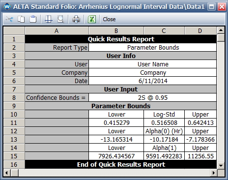
  • The 95% two-sided confidence bounds are: for [math]\displaystyle{ \sigma\,\! }[/math] it is [0.42, 0.64]; for [math]\displaystyle{ \beta_{0}\,\! }[/math] it is [-13.2, -7.2]; for [math]\displaystyle{ \beta_{1}\,\! }[/math] it is [0.68, 0.97]. In terms of [math]\displaystyle{ \alpha_{1}\,\! }[/math], the bounds are [7891.14, 11256.85].
  • The log-likelihood value is -88.26.
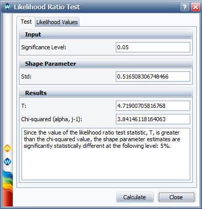
  • Common shape parameter test result: the likelihood ratio common shape parameter test statistic is 4.7. It is larger than the critical value 3.84. This indicates that there is some lack of fit in the constant [math]\displaystyle{ \sigma\,\! }[/math] assumption across all the stress levels.


Results in ALTA

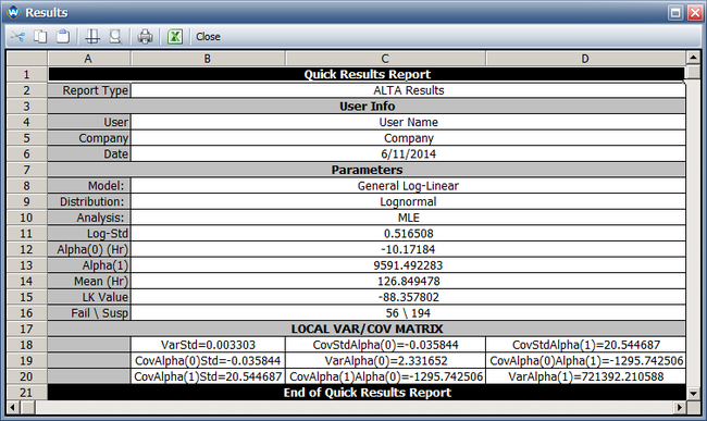
  • The following picture shows the ML estimations for the model parameters in ALTA and the log-likelihood value (LK Value).
Arrhenius Log results.png


The picture above also shows variance of each parameter. These are: [math]\displaystyle{ Var(\sigma)\,\! }[/math] = 0.003303,  [math]\displaystyle{ Var(\alpha_{0})\,\! }[/math] = 2.331652,  [math]\displaystyle{ Var(\alpha_{1})\,\! }[/math] = 721392.210588. In terms of [math]\displaystyle{ \beta_{1}\,\! }[/math] , the variance is [math]\displaystyle{ Var(\beta_{1}) = \frac{Var(\alpha_{1})}{11605^{2}}\,\! }[/math] = 0.0053565.

The differences in the variance in ALTA and the results in the book are caused by the precision in the book since results are provided only up to the 2nd decimal.

  • The 95% two-sided confidence bounds on the parameters are shown next:
Arrhenius Log parameter bounds.png


  • The likelihood ratio common shape parameter test statistic is 4.7, as shown next.
Arrhenius Log LK test.png


As the results show, the values obtained by ALTA are very close to the results given in the book.