Degradation Data Analysis with a Linear Regression Model: Difference between revisions

From ReliaWiki
Jump to navigation Jump to search
(Created page with '{{Reference Example}} This example compares the results for a degradation analysis with a linear regression model. {{Reference_Example_Heading1}} The data set is from Exampl…')
 
No edit summary
Line 74: Line 74:


{{Reference_Example_Heading4}}
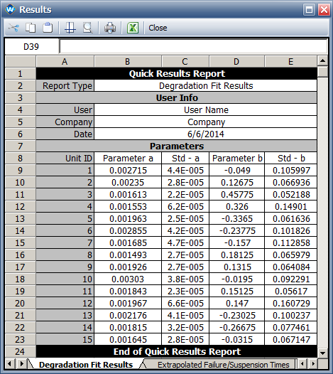
* For the power regression model
[[Image:DA_linear_model.png|center|]]
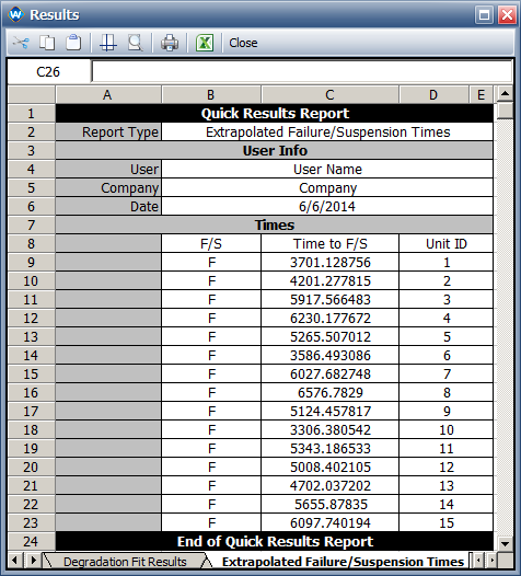
* The predicted pseudo failure times.
[[Image:DA_linear_extrapolated.png|center|]]
: The predicted failure times in Weibull++ are slightly different from the values given in the book. Since the book does not provide the model parameters, we couldn’t compare the Weibulll++ results with the results in the book.
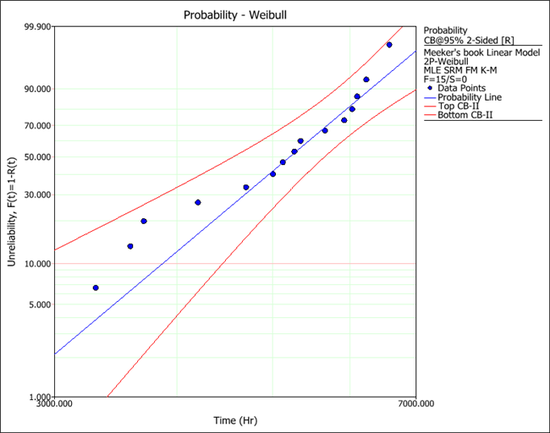
* The fitted Weibull distribution
[[Image:DA_linear_plot.png|center|550px|]]

Revision as of 18:41, 6 June 2014

Weibull Reference Examples Banner.png


New format available! This reference is now available in a new format that offers faster page load, improved display for calculations and images and more targeted search.

As of January 2024, this Reliawiki page will not continue to be updated. Please update all links and bookmarks to the latest references at Weibull examples and Weibull reference examples.

Degradation Data Analysis with a Linear Regression Model

This example compares the results for a degradation analysis with a linear regression model.


Reference Case

The data set is from Example 13.10 on page 338 in the book Statistical Methods for Reliability Data by Dr. Meeker and Dr. Escobar, John Wiley & Sons, 1998.


Data

The test is for the current (amperage) of a laser device. Failure is defined as a 10% increases in amperage.

Time Unit Number
1 2 3 4 5 6 7 8 9 10 11 12 13 14 15
250 0.47 0.71 0.71 0.36 0.27 0.36 0.36 0.46 0.51 0.41 0.44 0.4 0.3 0.44 0.51
500 0.93 1.22 1.17 0.62 0.61 1.39 0.92 1.07 0.93 1.79 1 0.8 0.74 0.7 0.83
750 2.11 1.9 1.73 1.36 1.11 1.95 1.21 1.42 1.57 2.38 1.57 1.4 1.52 1.05 1.29
1000 2.72 2.3 1.99 1.95 1.77 2.86 1.46 1.77 1.96 3 1.96 1.7 1.85 1.35 1.52
1250 3.51 2.87 2.53 2.3 2.06 3.46 1.93 2.11 2.59 3.84 2.51 3 2.39 1.8 1.91
1500 4.34 3.75 2.97 2.95 2.58 3.81 2.39 2.4 3.29 4.5 2.84 3.6 2.95 2.55 2.27
1750 4.91 4.42 3.3 3.39 2.99 4.53 2.68 2.78 3.61 5.25 3.47 4 3.51 2.83 2.78
2000 5.48 4.99 3.94 3.79 3.38 5.35 2.94 3.02 4.11 6.26 4.01 4.4 3.92 3.39 3.42
2250 5.99 5.51 4.16 4.11 4.05 5.92 3.42 3.29 4.6 7.05 4.51 4.8 5.03 3.72 3.78
2500 6.72 6.07 4.45 4.5 4.63 6.17 4.09 3.75 4.91 7.8 4.8 5.2 5.47 4.09 4.11
2750 7.13 6.64 4.89 4.72 5.24 7.7 4.58 4.16 5.34 8.32 5.2 5.5 5.84 4.83 4.38
3000 8 7.16 5.27 4.98 5.62 8.61 4.84 4.76 5.84 8.93 5.66 6 6.5 5.41 4.63
3250 8.92 7.78 5.69 5.28 6.04 9.15 5.11 5.16 6.4 9.55 6.2 6.2 6.94 5.76 5.38
3500 9.49 8.42 6.02 5.61 6.32 9.95 5.57 5.46 6.84 10.5 6.54 7 7.39 6.14 5.84
3750 9.87 8.91 6.45 5.95 7.1 10.49 6.11 5.81 7.2 11.3 6.96 7.4 7.85 6.51 6.16
4000 10.94 9.28 6.88 6.14 7.59 11.01 7.17 6.24 7.88 12.2 7.42 7.9 8.09 6.88 6.62


Result

The book provides a linear regression model, [math]\displaystyle{ y=b+at\,\! }[/math], but the parameters of the model are not provided. Only the predicted failure times are given. These are: 3702, 4194, 5847, 6172, 5301, 3592, 6051, 6538, 5110, 3306, 5326, 4995, 4721, 5689, and 6102. A Weibull distribution is used to fit the data; however, the model parameters are not provided. Only a probability plot is given.


Results in Weibull++

  • For the power regression model
DA linear model.png


  • The predicted pseudo failure times.
DA linear extrapolated.png


The predicted failure times in Weibull++ are slightly different from the values given in the book. Since the book does not provide the model parameters, we couldn’t compare the Weibulll++ results with the results in the book.


  • The fitted Weibull distribution
DA linear plot.png