Maintenance Planning

For components and systems with increasing failure rate, planned replacements and inspections are often used to prevent failures in order to improve system availability and reduce overall maintenance cost. For example, the common used preventive maintenance strategy is to replace an aged item at a given time interval in order to minimize the long term cost per unit time. An optimal time interval exists if the failure rate is creasing and the cost of failure is much higher than the cost of a scheduled replacement. Another alternative is to minimize the short term cost per unit time, such as in one maintenance cycle. A replacement cycle is defined as the time when a failure occurs or at the scheduled replacement if there is no failure. Similarly, periodical inspection is applied to detect a potential failure and to prevent its happening. The objective of inspection also can be to minimize either the long time or the short time cost. In this section, we will discuss how to find the optimal maintenance and inspection intervals in order to minimize the long term and the short term maintenance cost.

Optimal Preventive Replacement Interval

Minimize the Long Term Cost Per Unit Time

Minimizing the long term maintenance cost per unit time is the most popular objective for adopting a preventive replacement strategy. The theory behind this strategy is discussed in the Systems Reliability Analysis Reference book, but we will provide a brief explanation here.

For an item that is either replaced at the time of failure or at the time of the scheduled maintenance interval [math]\displaystyle{ x }[/math], the expected cycle length is:

[math]\displaystyle{ E(\text{Cycle Length})=\int_{0}^{x}{tf(t)dt}+R(x)x=\int_{0}^{x}{R(t)dt} }[/math]

The expected cost for one cycle is:

[math]\displaystyle{ E(\text{Cost Per Cycle})={{C}_{P}}R(x)+{{C}_{U}}\left( 1-R(x) \right) }[/math]

Therefore, the expected long term cost per unit time is:

[math]\displaystyle{ CPU{{T}_{L}}(t)=\frac{E(\text{Cost Per Cycle})}{E\left( \text{Cycle Length} \right)}=\frac{{{C}_{P}}R(x)+{{C}_{U}}\left( 1-R(x) \right)}{\int_{0}^{x}{R(t)dt}} }[/math]

The optimal preventive maintenance interval will be the value t which minimizes [math]\displaystyle{ CPU{{T}_{L}} }[/math]. In the above equations:

• [math]\displaystyle{ f(x) }[/math] is the probability density function of the failure time.
• [math]\displaystyle{ R(x) }[/math] is the reliability function of the failure time.
• [math]\displaystyle{ {{C}_{P}} }[/math] is the average cost due to a planned maintenance.
• [math]\displaystyle{ {{C}_{U}} }[/math] is the average cost due to a unplanned maintenance.

Minimize the Short Term Cost Per Unit Time

The equations above are based on the reward renewal theory and are used for minimizing the long term maintenance cost. There may be cases, however, where the average costs change with time, or when components are replaced with either costlier or less expensive versions. In this situation, the failure time distribution and the cost function need to be updated every time the costs change. Therefore, an optimal interval to minimize the short term cost is needed.

The expected cost per unit time in one replacement cycle is defined as:

[math]\displaystyle{ CPU{{T}_{S}}(t)=E\left( \frac{\text{Cost Per Cycle}}{\text{Cycle Length}} \right)=\int_{0}^{x}{\frac{{{C}_{U}}}{t}f(t)dt}+\frac{{{C}_{P}}}{x}\left( 1-F(x) \right) }[/math]

For a Weibull distribution with its shape parameter [math]\displaystyle{ \beta \gt 1 }[/math], the optimal interval [math]\displaystyle{ {{x}_{0}} }[/math] is:

[math]\displaystyle{ {{x}_{o}}=\eta {{\left( \frac{{{C}_{P}}}{\beta \left( {{C}_{U}}-{{C}_{P}} \right)} \right)}^{\frac{1}{\beta }}} }[/math]

where [math]\displaystyle{ \eta }[/math] is the scale parameter of the Weibull distribution.

Optimal Inspection Interval

Inspection is often used to test if a device is working properly. For example, signs of a device's impending failure due to degradation, such as corrosion, can be detected via inspection. The device can then be replaced before the failure actually occurs. If a failure cannot be detected during the inspection, it will be noticed immediately when the failure occurs, and the device will be replaced at the time of the failure.

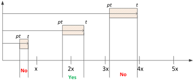
Assume that a failure occurs at time [math]\displaystyle{ t }[/math]. If an inspection is conducted within the range of [math]\displaystyle{ [p\times t,t] }[/math], the failure will be detected and the component will be replaced. The term p is a value between 0 and 1. This is illustrated in the following plot.

In the plot, the inspection is conducted at every X hours. "No" means that an oncoming failure will not be detected by inspection, while "Yes" means it can be detected by inspection since the inspection time is within [math]\displaystyle{ [p\times t,t] }[/math]. In this case, whenever a replacement occurs, a new maintenance cycle starts.

Minimize the Long Term Cost Per Unit Time

Define:

M is the largest inspection interval where there is no overlap between the detection zones of two adjunct inspections. Any failures that occur after the Mth inspection will always be detected.

The expected replacement cycle length is:

[math]\displaystyle{ \begin{align} & E(\text{Cycle Length})=\int_{0}^{x}{{{C}_{U}}f(t)dt}+\sum\limits_{k=1}^{M}{\left[ \int\limits_{kx}^{\frac{kx}{p}}{\left[ {{C}_{P}}+k{{C}_{I}} \right]}f(t)dt+\int\limits_{\frac{kx}{p}}^{(k+1)x}{\left[ {{C}_{U}}+k{{C}_{I}} \right]}f(t)dt \right]} \\ & +\int\limits_{\left( M+1 \right)x}^{\frac{(M+1)x}{p}}{\left[ {{C}_{P}}+(M+1){{C}_{I}} \right]}f(t)dt+\sum\limits_{k=M+1}^{\infty }{\int\limits_{\frac{kx}{p}}^{\frac{(k+1)x}{p}}{\left[ {{C}_{P}}+(k+1){{C}_{I}} \right]f(t)dt}} \end{align} }[/math]

The expected cost for one cycle is:

[math]\displaystyle{ \begin{align} & E(\text{Cost Per Cycle})=\int_{0}^{x}{tf(t)dt}+\sum\limits_{k=1}^{M}{\left[ \int\limits_{kx}^{\frac{kx}{p}}{\left( kx \right)}f(t)dt+\int\limits_{\frac{kx}{p}}^{(k+1)x}{t}f(t)dt \right]} \\ & +\int\limits_{\left( M+1 \right)x}^{\frac{(M+1)x}{p}}{\left[ (M+1)x \right]}f(t)dt+\sum\limits_{k=M+1}^{\infty }{\int\limits_{\frac{kx}{p}}^{\frac{(k+1)x}{p}}{\left[ (k+1)x \right]f(t)dt}} \end{align} }[/math]

The expected long term cost per unit time is:

[math]\displaystyle{ CPU{{T}_{L}}(t)=\frac{E(\text{Cost Per Cycle})}{E\left( \text{Cycle Length} \right)} }[/math]

where [math]\displaystyle{ {{C}_{I}} }[/math] is the average cost per inspection.

Minimize the Short Term Cost Per Unit Time

The short term (one replacement cycle) cost per unit time is:

[math]\displaystyle{ \begin{align} & CPU{{T}_{S}}=E\left( \frac{\text{Cost per Cycle}}{\text{Cycle Length}} \right)=\int_{0}^{x}{\frac{{{C}_{U}}}{t}f(t)dt} \\ & +\sum\limits_{k=1}^{M}{\left[ \int\limits_{kx}^{\frac{kx}{p}}{\frac{{{C}_{P}}+k{{C}_{I}}}{kx}}f(t)dt+\int\limits_{\frac{kx}{p}}^{(k+1)x}{\frac{{{C}_{U}}+k{{C}_{I}}}{t}}f(t)dt \right]} \\ & +\int\limits_{\left( M+1 \right)x}^{\frac{(M+1)x}{p}}{\frac{{{C}_{P}}+(M+1){{C}_{I}}}{(M+1)x}}f(t)dt+\sum\limits_{k=M+1}^{\infty }{\int\limits_{\frac{kx}{p}}^{\frac{(k+1)x}{p}}{\frac{{{C}_{P}}+(k+1){{C}_{I}}}{(k+1)x}f(t)dt}} \\ \end{align} }[/math]

Example

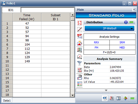
Assume that we are going to use the Maintenance Planning tool in Weibull++ to analyze a device that is assembled as part of a system. The failure times of the device are recorded and a Weibull distribution is used to model the data. The following picture shows the Weibull++ standard folio that contains the data and distribution. The Weibull distribution has parameters [math]\displaystyle{ \beta\,\! }[/math] = 2.847494 and [math]\displaystyle{ \eta\,\! }[/math] = 108.420135.

Assume that the average cost for a planned replacement of the device is $20. For an unplanned replacement, the cost is $500. The cost for each inspection is $10, and the fraction of the failure time for detecting an oncoming failure is 0.9. The objectives are:

• Find the optimal inspection interval and the optimal scheduled replacement interval for minimizing the cost in the long term.
• Find the optimal inspection interval and the optimal scheduled replacement interval for minimizing the cost in one replacement cycle.

Solution

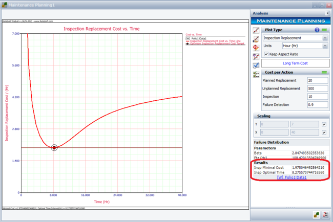
In the Maintenance Planning tool, choose the Inspection Replacement plot type on the control panel, and then enter the estimated costs. Click the Plot icon to calculate the results and draw the plot. The following results show that the optimal inspection interval is about 8.28 hours, and the minimal cost is about $1.98 per hour.

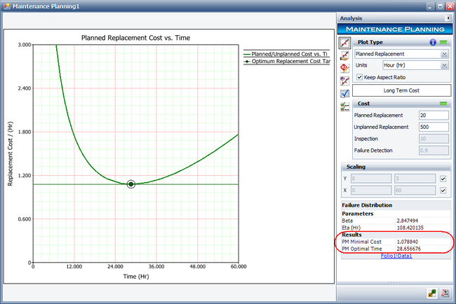
To use a scheduled replacement strategy, choose the Planned Replacement plot type on the control panel, and then click the Plot icon again to recalculate results and redraw the plot. The following results show that the optimal replacement interval is about 28.657 hours, and the minimal cost is about $1.079 per hour.

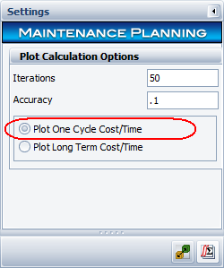
To find the optimal times for minimizing the cost in one replacement cycle, select the Plot One Cycle Cost/Time option on the Settings page of the control panel.

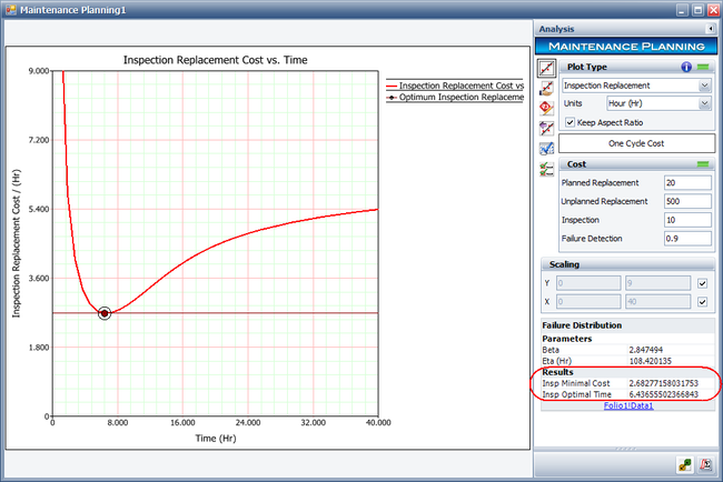
Next, choose the Inspection Replacement plot type on the Main page of the control panel and recalculate the results. The results show that the optimal inspection interval for one replacement cycle is about 6.437 hours, and the minimal cost is about $2.683 per hour.

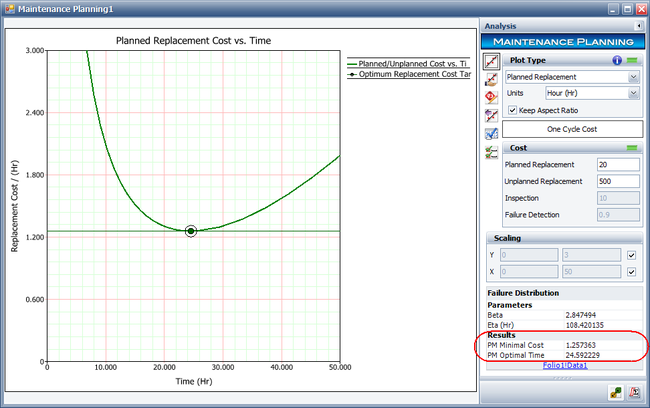
Change the plot type to Planned Replacement and recalculate the results. The results show that the optimal replacement interval is about 24.592 hours, and the minimal cost is about $1.257 per hour.

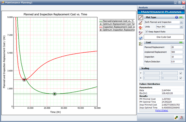
To plot both the planned replacement and inspection replacement plots, choose the Both Planned and Inspection plot type. The results are shown next.

Based on the above results, we can now make decisions about our maintenance strategy. For example, if our plan is to reduce the short term maintenance cost, then the device should be scheduled for replacement at about every 24 hours. This will give us a minimal maintenance cost of $1.257 per hour.