Generalized Eyring Relationship: Difference between revisions
Chris Kahn (talk | contribs) (Created page with '<noinclude>{{Navigation box}} ''This article also appears in the Accelerated Life Testing Data Analysis Reference book.'' </noinclude> The generalized Eyr…') |
Chris Kahn (talk | contribs) No edit summary |
||
| Line 1: | Line 1: | ||
<noinclude>{{Navigation box}} | <noinclude>{{Navigation box}} | ||
''This article also appears in the [[Eyring Relationship|Accelerated Life Testing Data Analysis Reference]] book.'' </noinclude> | ''This article also appears in the [[Eyring Relationship|Accelerated Life Testing Data Analysis Reference]] book.'' </noinclude> | ||
The generalized Eyring relationship is used when temperature and a second non-thermal stress (e.g. voltage) are the accelerated stresses of a test and their interaction is also of interest. This relationship is given by: | The generalized Eyring relationship is used when temperature and a second non-thermal stress (e.g. voltage) are the accelerated stresses of a test and their interaction is also of interest. This relationship is given by: | ||
Latest revision as of 22:17, 25 January 2013
This article also appears in the Accelerated Life Testing Data Analysis Reference book.
The generalized Eyring relationship is used when temperature and a second non-thermal stress (e.g. voltage) are the accelerated stresses of a test and their interaction is also of interest. This relationship is given by:
- [math]\displaystyle{ L(V,U)=\frac{1}{V}{{e}^{A+\tfrac{B}{V}+CU+D\tfrac{U}{V}}}\,\! }[/math]
where:
- [math]\displaystyle{ V\,\! }[/math] is the temperature (in absolute units).
- [math]\displaystyle{ U\,\! }[/math] is the non-thermal stress (i.e., voltage, vibration, etc.).
[math]\displaystyle{ A,B,C,D\,\! }[/math] are the parameters to be determined.
The Eyring relationship is a simple case of the generalized Eyring relationship where [math]\displaystyle{ C=D=0\,\! }[/math] and [math]\displaystyle{ {{A}_{Eyr}}=-{{A}_{GEyr}}.\,\! }[/math] Note that the generalized Eyring relationship includes the interaction term of [math]\displaystyle{ U\,\! }[/math] and [math]\displaystyle{ V\,\! }[/math] as described by the [math]\displaystyle{ D\tfrac{U}{V}\,\! }[/math] term. In other words, this model can estimate the effect of changing one of the factors depending on the level of the other factor.
Acceleration Factor
Most models in actual use do not include any interaction terms, therefore, the acceleration factor can be computed by multiplying the acceleration factors obtained by changing each factor while keeping the other factors constant. In the case of the generalized Eyring relationship, the acceleration factor is derived differently.
The acceleration factor for the generalized Eyring relationship is given by:
- [math]\displaystyle{ \begin{align} & {{A}_{F}}= & \frac{{{L}_{USE}}}{{{L}_{Accelerated}}}=\frac{\tfrac{1}{{{V}_{U}}}{{e}^{A+\tfrac{B}{{{V}_{U}}}+C{{U}_{U}}+D\tfrac{{{U}_{U}}}{{{V}_{U}}}}}}{\tfrac{1}{{{T}_{A}}}{{e}^{A+\tfrac{B}{{{V}_{A}}}+C{{U}_{A}}+D\tfrac{{{U}_{A}}}{{{V}_{A}}}}}} =\ \frac{\tfrac{1}{{{V}_{U}}}{{e}^{A+\tfrac{B}{{{V}_{U}}}+C{{U}_{U}}+D\tfrac{{{U}_{U}}}{{{V}_{U}}}}}}{\tfrac{1}{{{V}_{A}}}{{e}^{A+\tfrac{B}{{{V}_{A}}}+C{{U}_{A}}+D\tfrac{{{U}_{A}}}{{{V}_{A}}}}}} \end{align}\,\! }[/math]
where:
- [math]\displaystyle{ {{L}_{USE}}\,\! }[/math] is the life at use stress level.
- [math]\displaystyle{ {{L}_{Accelerated}}\,\! }[/math] is the life at the accelerated stress level.
- [math]\displaystyle{ {{V}_{u}}\,\! }[/math] is the use temperature level.
- [math]\displaystyle{ {{V}_{A}}\,\! }[/math] is the accelerated temperature level.
- [math]\displaystyle{ {{U}_{A}}\,\! }[/math] is the accelerated non-thermal level.
- [math]\displaystyle{ {{U}_{u}}\,\! }[/math] is the use non-thermal level.
Generalized Eyring-Exponential
By setting [math]\displaystyle{ m=L(V,U)\,\! }[/math], the exponential pdf becomes:
- [math]\displaystyle{ f(t,V,U)=\left( V{{e}^{-A-\tfrac{B}{V}-CU-D\tfrac{U}{V}}} \right){{e}^{-tV{{e}^{-A-\tfrac{B}{V}-CU-D\tfrac{U}{V}}}}}\,\! }[/math]
Generalized Eyring-Exponential Reliability Function
The generalized Eyring exponential model reliability function is given by:
- [math]\displaystyle{ R(T,U,V)={{e}^{-tV{{e}^{-A-\tfrac{B}{V}-CU-D\tfrac{U}{V}}}}}\,\! }[/math]
Parameter Estimation
Substituting the generalized Eyring model into the lognormal log-likelihood equation yields:
- [math]\displaystyle{ \begin{align} & \ln (L)= & \Lambda =\overset{Fe}{\mathop{\underset{i=1}{\mathop{\underset{}{\overset{}{\mathop \sum }}\,}}\,}}\,{{N}_{i}}\ln [\frac{\varphi (z(t))}{\sigma _{T}^{\prime }t}]\overset{S}{\mathop{\underset{i=1}{\mathop{+\underset{}{\overset{}{\mathop \sum }}\,}}\,}}\,N_{i}^{\prime }\ln \left( 1-\Phi (z(t_{i}^{\prime })) \right) +\overset{FI}{\mathop{\underset{i=1}{\mathop{\underset{}{\overset{}{\mathop \sum }}\,}}\,}}\,N_{i}^{\prime \prime }\ln [\Phi (z_{Ri}^{\prime \prime })-\Phi (z_{Li}^{\prime \prime })] \end{align}\,\! }[/math]
where:
- [math]\displaystyle{ z_{Ri}^{\prime \prime }=\frac{\ln t_{Ri}^{\prime \prime }-A-\tfrac{B}{V_{i}^{\prime \prime }}-C{{U}_{i}}-D\tfrac{{{U}_{i}}}{V_{i}^{\prime \prime }}+\ln (V_{i}^{\prime \prime })}{\sigma _{T}^{\prime }}\,\! }[/math]
- [math]\displaystyle{ z_{Li}^{\prime \prime }=\frac{\ln t_{Ri}^{\prime \prime }-A-\tfrac{B}{V_{i}^{\prime \prime }}-C{{U}_{i}}-D\tfrac{{{U}_{i}}}{V_{i}^{\prime \prime }}+\ln (V_{i}^{\prime \prime })}{\sigma _{T}^{\prime }}\,\! }[/math]
and:
- [math]\displaystyle{ {{F}_{e}}\,\! }[/math] is the number of groups of exact times-to-failure data points.
- [math]\displaystyle{ {{N}_{i}}\,\! }[/math] is the number of times-to-failure data points in the [math]\displaystyle{ {{i}^{th}}\,\! }[/math] time-to-failure data group.
- [math]\displaystyle{ A,B,C,D\,\! }[/math] are parameters to be estimated.
- [math]\displaystyle{ {{V}_{i}}\,\! }[/math] is the temperature level of the [math]\displaystyle{ {{i}^{th}}\,\! }[/math] group.
- [math]\displaystyle{ {{U}_{i}}\,\! }[/math] is the non-thermal stress level of the [math]\displaystyle{ {{i}^{th}}\,\! }[/math] group.
- [math]\displaystyle{ {{T}_{i}}\,\! }[/math] is the exact failure time of the [math]\displaystyle{ {{i}^{th}}\,\! }[/math] group.
- [math]\displaystyle{ S\,\! }[/math] is the number of groups of suspension data points.
- [math]\displaystyle{ N_{i}^{\prime }\,\! }[/math] is the number of suspensions in the [math]\displaystyle{ {{i}^{th}}\,\! }[/math] group of suspension data points.
- [math]\displaystyle{ T_{i}^{\prime }\,\! }[/math] is the running time of the [math]\displaystyle{ {{i}^{th}}\,\! }[/math] suspension data group.
- [math]\displaystyle{ FI\,\! }[/math] is the number of interval data groups.
- [math]\displaystyle{ N_{i}^{\prime \prime }\,\! }[/math] is the number of intervals in the [math]\displaystyle{ {{i}^{th}}\,\! }[/math] group of data intervals.
- [math]\displaystyle{ T_{Li}^{\prime \prime }\,\! }[/math] is the beginning of the [math]\displaystyle{ {{i}^{th}}\,\! }[/math] interval.
- [math]\displaystyle{ T_{Ri}^{\prime \prime }\,\! }[/math] is the ending of the [math]\displaystyle{ {{i}^{th}}\,\! }[/math] interval.
The solution (parameter estimates) will be found by solving for the parameters [math]\displaystyle{ A,\,\! }[/math] [math]\displaystyle{ B,\,\! }[/math] [math]\displaystyle{ C,\,\! }[/math] and [math]\displaystyle{ D\,\! }[/math] so that [math]\displaystyle{ \tfrac{\partial \Lambda }{\partial A}=0,\,\! }[/math] [math]\displaystyle{ \tfrac{\partial \Lambda }{\partial B}=0,\,\! }[/math] [math]\displaystyle{ \tfrac{\partial \Lambda }{\partial D}=0\,\! }[/math] and [math]\displaystyle{ \tfrac{\partial \Lambda }{\partial D}=0\,\! }[/math].
Generalized Eyring-Weibull
By setting [math]\displaystyle{ \eta =L(V,U)\,\! }[/math] to the Weibull pdf, the generalized Eyring Weibull model is given by:
- [math]\displaystyle{ \begin{align} & f(t,V,U)= & \beta \left( V{{e}^{-A-\tfrac{B}{V}-CU-D\tfrac{U}{V}}} \right){{\left( tV{{e}^{-A-\tfrac{B}{V}-CU-D\tfrac{U}{V}}} \right)}^{\beta -1}} {{e}^{-{{\left( tV{{e}^{-A-\tfrac{B}{V}-CU-D\tfrac{U}{V}}} \right)}^{\beta }}}} \end{align}\,\! }[/math]
Generalized Eyring-Weibull Reliability Function
The generalized Eyring Weibull reliability function is given by:
- [math]\displaystyle{ R(T,V,U)={{e}^{-{{\left( tV{{e}^{-A-\tfrac{B}{V}-CU-D\tfrac{U}{V}}} \right)}^{\beta }}}}\,\! }[/math]
Parameter Estimation
Substituting the generalized Eyring model into the Weibull log-likelihood equation yields:
- [math]\displaystyle{ \begin{align} \ln (L)= \Lambda = & \overset{Fe}{\mathop{\underset{i=1}{\mathop{\underset{}{\overset{}{\mathop \sum }}\,}}\,}}\,{{N}_{i}}\ln [\beta \left( V{{e}^{-A-\tfrac{B}{V}-CU-D\tfrac{U}{V}}} \right) {{\left( tV{{e}^{-A-\tfrac{B}{V}-CU-D\tfrac{U}{V}}} \right)}^{\beta -1}}] -\overset{Fe}{\mathop{\underset{i=1}{\mathop{\underset{}{\overset{}{\mathop \sum }}\,}}\,}}\,{{N}_{i}}{{\left( {{t}_{i}}{{V}_{i}}{{e}^{-A-\tfrac{B}{{{V}_{i}}}-C{{U}_{i}}-D\tfrac{{{U}_{i}}}{{{V}_{i}}}}} \right)}^{\beta }} \\ & -\overset{S}{\mathop{\underset{i=1}{\mathop{\underset{}{\overset{}{\mathop \sum }}\,}}\,}}\,N_{i}^{\prime }{{\left( t_{i}^{\prime }V_{i}^{\prime }{{e}^{-A-\tfrac{B}{V_{i}^{\prime }}-CU_{i}^{\prime }-D\tfrac{U_{i}^{\prime }}{V_{i}^{\prime }}}} \right)}^{\beta }} +\overset{FI}{\mathop{\underset{i=1}{\mathop{\underset{}{\overset{}{\mathop \sum }}\,}}\,}}\,N_{i}^{\prime \prime }\ln [R_{Li}^{\prime \prime }-R_{Ri}^{\prime \prime }] \end{align}\,\! }[/math]
where:
- [math]\displaystyle{ R_{Li}^{\prime \prime }(T_{Li}^{\prime \prime })={{e}^{-{{\left( T_{Li}^{\prime \prime }V_{i}^{\prime \prime }{{e}^{-A-\tfrac{B}{V_{i}^{\prime \prime }}-C{{U}_{i}}-D\tfrac{{{U}_{i}}}{V_{i}^{\prime \prime }}}} \right)}^{\beta }}}}\,\! }[/math]
- [math]\displaystyle{ R_{Ri}^{\prime \prime }(T_{Ri}^{\prime \prime })={{e}^{-{{\left( T_{Ri}^{\prime \prime }V_{i}^{\prime \prime }{{e}^{-A-\tfrac{B}{V_{i}^{\prime \prime }}-C{{U}_{i}}-D\tfrac{{{U}_{i}}}{V_{i}^{\prime \prime }}}} \right)}^{\beta }}}}\,\! }[/math]
and:
- [math]\displaystyle{ {{F}_{e}}\,\! }[/math] is the number of groups of exact times-to-failure data points.
- [math]\displaystyle{ {{N}_{i}}\,\! }[/math] is the number of times-to-failure data points in the [math]\displaystyle{ {{i}^{th}}\,\! }[/math] time-to-failure data group.
- [math]\displaystyle{ A,B,C,D\,\! }[/math] are parameters to be estimated.
- [math]\displaystyle{ {{V}_{i}}\,\! }[/math] is the temperature level of the [math]\displaystyle{ {{i}^{th}}\,\! }[/math] group.
- [math]\displaystyle{ {{U}_{i}}\,\! }[/math] is the non-thermal stress level of the [math]\displaystyle{ {{i}^{th}}\,\! }[/math] group.
- [math]\displaystyle{ {{T}_{i}}\,\! }[/math] is the exact failure time of the [math]\displaystyle{ {{i}^{th}}\,\! }[/math] group.
- [math]\displaystyle{ S\,\! }[/math] is the number of groups of suspension data points.
- [math]\displaystyle{ N_{i}^{\prime }\,\! }[/math] is the number of suspensions in the [math]\displaystyle{ {{i}^{th}}\,\! }[/math] group of suspension data points.
- [math]\displaystyle{ T_{i}^{\prime }\,\! }[/math] is the running time of the [math]\displaystyle{ {{i}^{th}}\,\! }[/math] suspension data group.
- [math]\displaystyle{ FI\,\! }[/math] is the number of interval data groups.
- [math]\displaystyle{ N_{i}^{\prime \prime }\,\! }[/math] is the number of intervals in the [math]\displaystyle{ {{i}^{th}}\,\! }[/math] group of data intervals.
- [math]\displaystyle{ T_{Li}^{\prime \prime }\,\! }[/math] is the beginning of the [math]\displaystyle{ {{i}^{th}}\,\! }[/math] interval.
- [math]\displaystyle{ T_{Ri}^{\prime \prime }\,\! }[/math] is the ending of the [math]\displaystyle{ {{i}^{th}}\,\! }[/math] interval.
The solution (parameter estimates) will be found by solving for the parameters [math]\displaystyle{ A,\,\! }[/math] [math]\displaystyle{ B,\,\! }[/math] [math]\displaystyle{ C,\,\! }[/math] and [math]\displaystyle{ D\,\! }[/math] so that [math]\displaystyle{ \tfrac{\partial \Lambda }{\partial A}=0,\,\! }[/math] [math]\displaystyle{ \tfrac{\partial \Lambda }{\partial B}=0,\,\! }[/math] [math]\displaystyle{ \tfrac{\partial \Lambda }{\partial D}=0\,\! }[/math] and [math]\displaystyle{ \tfrac{\partial \Lambda }{\partial D}=0\,\! }[/math].
Generalized Eyring-Lognormal
By setting [math]\displaystyle{ \sigma _{T}^{\prime }=L(V,U)\,\! }[/math] to the lognormal pdf, the generalized Erying lognormal model is given by:
- [math]\displaystyle{ f(t,V,U)=\frac{\varphi (z(t))}{\sigma _{T}^{\prime }t}\,\! }[/math]
where:
- [math]\displaystyle{ z(t)=\frac{\ln t-A-\tfrac{B}{V}-CU-D\tfrac{U}{V}+\ln (V)}{\sigma _{T}^{\prime }}\,\! }[/math]
Generalized Eyring-Lognormal Reliability Function
The generalized Erying lognormal reliability function is given by:
- [math]\displaystyle{ \begin{align} R(T,V,U)=1-\Phi (z) \end{align}\,\! }[/math]
Parameter Estimation
Substituting the generalized Eyring model into the lognormal log-likelihood equation yields:
- [math]\displaystyle{ \begin{align} & \ln (L)= & \Lambda =\overset{Fe}{\mathop{\underset{i=1}{\mathop{\underset{}{\overset{}{\mathop \sum }}\,}}\,}}\,{{N}_{i}}\ln [\frac{\varphi (z(t))}{\sigma _{T}^{\prime }t}]\overset{S}{\mathop{\underset{i=1}{\mathop{+\underset{}{\overset{}{\mathop \sum }}\,}}\,}}\,N_{i}^{\prime }\ln \left( 1-\Phi (z(t_{i}^{\prime })) \right) +\overset{FI}{\mathop{\underset{i=1}{\mathop{\underset{}{\overset{}{\mathop \sum }}\,}}\,}}\,N_{i}^{\prime \prime }\ln [\Phi (z_{Ri}^{\prime \prime })-\Phi (z_{Li}^{\prime \prime })] \end{align}\,\! }[/math]
where:
- [math]\displaystyle{ z_{Ri}^{\prime \prime }=\frac{\ln t_{Ri}^{\prime \prime }-A-\tfrac{B}{V_{i}^{\prime \prime }}-C{{U}_{i}}-D\tfrac{{{U}_{i}}}{V_{i}^{\prime \prime }}+\ln (V_{i}^{\prime \prime })}{\sigma _{T}^{\prime }}\,\! }[/math]
- [math]\displaystyle{ z_{Li}^{\prime \prime }=\frac{\ln t_{Ri}^{\prime \prime }-A-\tfrac{B}{V_{i}^{\prime \prime }}-C{{U}_{i}}-D\tfrac{{{U}_{i}}}{V_{i}^{\prime \prime }}+\ln (V_{i}^{\prime \prime })}{\sigma _{T}^{\prime }}\,\! }[/math]
and:
- [math]\displaystyle{ {{F}_{e}}\,\! }[/math] is the number of groups of exact times-to-failure data points.
- [math]\displaystyle{ {{N}_{i}}\,\! }[/math] is the number of times-to-failure data points in the [math]\displaystyle{ {{i}^{th}}\,\! }[/math] time-to-failure data group.
- [math]\displaystyle{ A,B,C,D\,\! }[/math] are parameters to be estimated.
- [math]\displaystyle{ {{V}_{i}}\,\! }[/math] is the temperature level of the [math]\displaystyle{ {{i}^{th}}\,\! }[/math] group.
- [math]\displaystyle{ {{U}_{i}}\,\! }[/math] is the non-thermal stress level of the [math]\displaystyle{ {{i}^{th}}\,\! }[/math] group.
- [math]\displaystyle{ {{T}_{i}}\,\! }[/math] is the exact failure time of the [math]\displaystyle{ {{i}^{th}}\,\! }[/math] group.
- [math]\displaystyle{ S\,\! }[/math] is the number of groups of suspension data points.
- [math]\displaystyle{ N_{i}^{\prime }\,\! }[/math] is the number of suspensions in the [math]\displaystyle{ {{i}^{th}}\,\! }[/math] group of suspension data points.
- [math]\displaystyle{ T_{i}^{\prime }\,\! }[/math] is the running time of the [math]\displaystyle{ {{i}^{th}}\,\! }[/math] suspension data group.
- [math]\displaystyle{ FI\,\! }[/math] is the number of interval data groups.
- [math]\displaystyle{ N_{i}^{\prime \prime }\,\! }[/math] is the number of intervals in the [math]\displaystyle{ {{i}^{th}}\,\! }[/math] group of data intervals.
- [math]\displaystyle{ T_{Li}^{\prime \prime }\,\! }[/math] is the beginning of the [math]\displaystyle{ {{i}^{th}}\,\! }[/math] interval.
- [math]\displaystyle{ T_{Ri}^{\prime \prime }\,\! }[/math] is the ending of the [math]\displaystyle{ {{i}^{th}}\,\! }[/math] interval.
The solution (parameter estimates) will be found by solving for the parameters [math]\displaystyle{ A,\,\! }[/math] [math]\displaystyle{ B,\,\! }[/math] [math]\displaystyle{ C,\,\! }[/math] and [math]\displaystyle{ D\,\! }[/math] so that [math]\displaystyle{ \tfrac{\partial \Lambda }{\partial A}=0,\,\! }[/math] [math]\displaystyle{ \tfrac{\partial \Lambda }{\partial B}=0,\,\! }[/math] [math]\displaystyle{ \tfrac{\partial \Lambda }{\partial D}=0\,\! }[/math] and [math]\displaystyle{ \tfrac{\partial \Lambda }{\partial D}=0\,\! }[/math].
Generalized Eyring Example
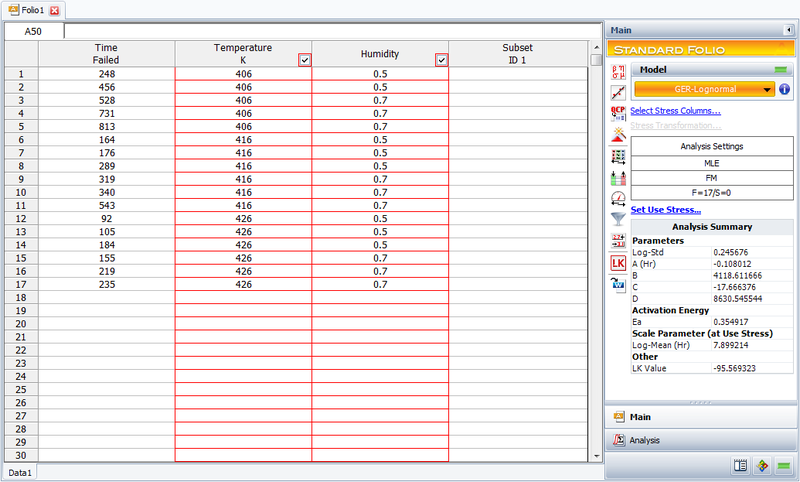
The following data set represents failure times (in hours) obtained from an electronics epoxy packaging accelerated life test performed to understand the synergy between temperature and humidity and estimate the [math]\displaystyle{ B10\,\! }[/math] life at the use conditions of [math]\displaystyle{ T=350K\,\! }[/math] and [math]\displaystyle{ H=0.3\,\! }[/math]. The data set is modeled using the lognormal distribution and the generalized Eyring model.
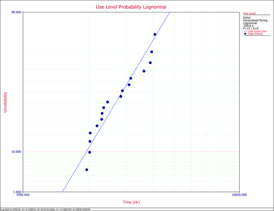
The probability plot at the use conditions is shown next.
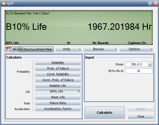
The [math]\displaystyle{ B10\,\! }[/math] information is estimated to be 1967.2 hours, as shown next.


