Highly Fractional Factorial Designs: Difference between revisions
Chris Kahn (talk | contribs) |
Chris Kahn (talk | contribs) No edit summary |
||
| Line 810: | Line 810: | ||
==Example== | ==Example== | ||
To illustrate single factor R-DOE analysis, consider the data in the table where life data readings for a product are taken at three levels of a certain factor, <math>A\,\!</math>. (Factor <math>A\,\!</math> may be thought of as a stress that is thought to affect life, three different designs of the same product, the same product manufactured by three different machines or operators, etc.) The goal of the experiment is to see if there is a change in life due to a change in the levels of the factor. The data | To illustrate single factor R-DOE analysis, consider the data in the table where life data readings for a product are taken at three levels of a certain factor, <math>A\,\!</math>. (Factor <math>A\,\!</math> may be thought of as a stress that is thought to affect life, three different designs of the same product, the same product manufactured by three different machines or operators, etc.) The goal of the experiment is to see if there is a change in life due to a change in the levels of the factor. The data from this experiment are shown in the figure below. | ||
| Line 816: | Line 816: | ||
The data is entered into a folio that is configured for | The data is entered into a folio that is configured for R-DOE analysis, as shown next. | ||
| Line 850: | Line 850: | ||
::<math>LR=-2\ln \frac{L({{{\hat{\theta }}}_{(-i)}})}{L(\hat{\theta })}\,\!</math> | |||
| Line 869: | Line 869: | ||
[[Image:doe11.11.png|thumb|center| | [[Image:doe11.11.png|thumb|center|650px|MLE results for the experiment in the [[Highly_Fractional_Factorial_Designs#Example_5| example]].]] | ||
| Line 900: | Line 900: | ||
If the null hypothesis, <math>{{H}_{0}}\,\!</math>, is true then the likelihood ratio will follow the | If the null hypothesis, <math>{{H}_{0}}\,\!</math>, is true then the likelihood ratio will follow the chi-squared distribution. The number of degrees of freedom for this distribution is equal to the difference in the number of parameters between the full and the reduced model. In this case, this difference is 2. The <math>p\,\!</math> value corresponding to the likelihood ratio on the chi-squared distribution with two degrees of freedom is: | ||
| Line 914: | Line 914: | ||
===Life Characteristic Summary Results=== | ===Life Characteristic Summary Results=== | ||
Results in the Life Characteristic Summary table | Results in the Life Characteristic Summary table include information about the life characteristic corresponding to each treatment level of the factor. If <math>\ln ({{\eta }_{i}})\,\!</math> is represented as <math>E({{y}_{i}})\,\!</math>, then the model for the life characteristic <math>\eta\,\!</math> can be written as: | ||
| Line 1,016: | Line 1,016: | ||
[[Image:doe11.12.png|thumb|center| | [[Image:doe11.12.png|thumb|center|650px|Life characteristic results for the experiment in the [[Highly_Fractional_Factorial_Designs#Example_5| example]].]] | ||
| Line 1,051: | Line 1,051: | ||
This is the value displayed by DOE++. Knowing the pooled standard error the confidence interval on the difference can be calculated. The 90% confidence interval on the difference in (logarithmic) life between levels 1 and 2 of factor <math>A\,\!</math> is: | This is the value displayed by DOE++. Knowing the pooled standard error, the confidence interval on the difference can be calculated. The 90% confidence interval on the difference in (logarithmic) life between levels 1 and 2 of factor <math>A\,\!</math> is: | ||
Revision as of 22:36, 17 October 2012
Reliability analysis is commonly thought of as an approach to model failures of existing products. The usual reliability analysis involves characterization of failures of the products using distributions such as exponential, Weibull and lognormal. Based on the fitted distribution, failures are mitigated, or warranty returns are predicted, or maintenance actions are planned. However, reliability analysis can also be used as a powerful tool to design robust products that operate with minimal failures, by adopting the methodology of Design for Reliability (DFR). In DFR, reliability analysis is carried out in conjunction with physics of failure and experiment design techniques. Under this approach, Design of Experiments (DOE) uses life data to "build" reliability into the products, not just quantify the existing reliability. Such an approach, if properly implemented, can result in significant cost savings, especially in terms of fewer warranty returns or repair and maintenance actions. Although DOE techniques can be used to improve product reliability and also make this reliability robust to noise factors, the discussion in this chapter is focused on reliability improvement.
Reliability DOE Analysis
Reliability DOE (R-DOE) analysis is fairly similar to the analysis of other designed experiments except that the response is the life of the product in the respective units (e.g., for an automobile component the units of life may be miles, for a mechanical component this may be cycles, and for a pharmaceutical product this may be months or years). However, two important differences exist that make R-DOE analysis unique. The first is that the life data of most products are typically well modeled by either the lognormal, Weibull or exponential distribution, but usually do not follow the normal distribution. Traditional DOE techniques follow the assumption that response values at any treatment level follow the normal distribution and therefore, the error terms, [math]\displaystyle{ \epsilon \,\! }[/math], can be assumed to be normally and independently distributed. This assumption may not be valid for the response data used in most of the R-DOE analyses. Further, the life data obtained may either be complete or censored, and in this case standard regression techniques applicable to the response data in traditional DOEs can no longer be used.
Stresses affecting the life of the product may also be investigated using R-DOE analysis. In this case, the primary purpose of any R-DOE analysis is to identify which of the investigated stresses affect the life of the product (by investigating if a change in the level of any stress leads to a significant change in the life of the product). Once the important stresses affecting the life of the product have been identified, detailed analyses can be carried out using ReliaSoft's ALTA software. ALTA includes a number of life-stress relationships (LSRs) to model the relation between life and the stress affecting the life of the product.
R-DOE Analysis of Lognormally Distributed Data
Assume that the life, [math]\displaystyle{ T\,\! }[/math], for a certain product has been found to be lognormally distributed. The probability density function for the lognormal distribution is:
- [math]\displaystyle{ f(T)=\frac{1}{T{\sigma }'\sqrt{2\pi }}{{e}^{-\frac{1}{2}{{\left( \frac{\ln (T)-{\mu }'}{{{\sigma }'}} \right)}^{2}}}}\,\! }[/math]
where [math]\displaystyle{ {\mu }'\,\! }[/math] represents the mean of the natural logarithm of the times-to-failure and [math]\displaystyle{ {\sigma }'\,\! }[/math] represents the standard deviation of the natural logarithms of the times-to-failure [Life Data Analysis Reference]. If the analyst wants to investigate a single two level factor that may affect the life, [math]\displaystyle{ T\,\! }[/math], then the following model may be used:
- [math]\displaystyle{ {{T}_{i}}={{\mu }_{i}}+{{\xi }_{i}}\,\! }[/math]
where:
- [math]\displaystyle{ {{T}_{i}}\,\! }[/math] represents the times-to-failure at the [math]\displaystyle{ i\,\! }[/math]th treatment level of the factor
- [math]\displaystyle{ {{\mu }_{i}}\,\! }[/math] represents the mean value of [math]\displaystyle{ {{T}_{i}}\,\! }[/math] for the [math]\displaystyle{ i\,\! }[/math]th treatment
- [math]\displaystyle{ {{\xi }_{i}}\,\! }[/math] is the random error term
- The subscript [math]\displaystyle{ i\,\! }[/math] represents the treatment level of the factor with [math]\displaystyle{ i=1,2\,\! }[/math] for a two level factor
The model of the equation given above is analogous to the ANOVA model, [math]\displaystyle{ {{Y}_{i}}={{\mu }_{i}}+{{\epsilon }_{i}}\,\! }[/math], used in Two Level Factorial Experiments for traditional DOE analyses. Note, however, that the random error term, [math]\displaystyle{ {{\xi }_{i}}\,\! }[/math], is not normally distributed here because the response, [math]\displaystyle{ T\,\! }[/math], is lognormally distributed. It is known that the logarithmic value of a lognormally distributed random variable follows the normal distribution. Therefore, if the logarithmic transformation of [math]\displaystyle{ T\,\! }[/math], [math]\displaystyle{ ln(T)\,\! }[/math], is used, the model will be identical to the ANOVA model, [math]\displaystyle{ {{Y}_{i}}={{\mu }_{i}}+{{\epsilon }_{i}}\,\! }[/math], used in two level factorial experiments. Thus, using the logarithmic failure times, the model can be written as:
- [math]\displaystyle{ \ln ({{T}_{i}})=\mu _{i}^{\prime }+{{\epsilon }_{i}}\,\! }[/math]
where:
- [math]\displaystyle{ \ln ({{T}_{i}})\,\! }[/math] represents the logarithmic times-to-failure at the [math]\displaystyle{ i\,\! }[/math]th treatment
- [math]\displaystyle{ \mu _{i}^{\prime }\,\! }[/math] represents the mean of the natural logarithm of the times-to-failure at the [math]\displaystyle{ i\,\! }[/math]th treatment
- [math]\displaystyle{ {\sigma }'\,\! }[/math] represents the standard deviation of the natural logarithms of the times-to-failure
The random error term, [math]\displaystyle{ {{\epsilon }_{i}}\,\! }[/math], is normally distributed because the response, [math]\displaystyle{ \ln ({{T}_{i}})\,\! }[/math], is normally distributed. Since the model of the equation given above is identical to the ANOVA model used in traditional DOE analysis, regression techniques can be applied here and the R-DOE analysis can be carried out similar to the traditional DOE analyses. Recall from Two Level factorial Experiments that if the factor(s) affecting the response has only two levels, then the notation of the regression model can be applied to the ANOVA model. Therefore, the model of can be written using a single indicator variable, [math]\displaystyle{ {{x}_{1}}\,\! }[/math], to represent the two level factor as:
- [math]\displaystyle{ \ln ({{T}_{i}})={{\beta }_{0}}+{{\beta }_{1}}{{x}_{i1}}+{{\epsilon }_{i}}\,\! }[/math]
where [math]\displaystyle{ {{\beta }_{0\text{ }}}\,\! }[/math] is the intercept term and [math]\displaystyle{ {{\beta }_{1}}\,\! }[/math] is the effect coefficient for the investigated factor. Setting the two equations given above equal to each other returns:
- [math]\displaystyle{ \mu _{i}^{\prime }={{\beta }_{0}}+{{\beta }_{1}}{{x}_{i1}}\,\! }[/math]
The natural logarithm of the times-to-failure at any factor level, [math]\displaystyle{ \mu _{i}^{\prime }\,\! }[/math], is referred to as the life characteristic because it represents a characteristic point of the underlying life distribution. The life characteristic used in the R-DOE analysis will change based on the underlying distribution assumed for the life data. If the analyst wants to investigate the effect of two factors (each at two levels) on the life of the product, then the life characteristic equation can be easily expanded as follows:
- [math]\displaystyle{ \mu _{i}^{\prime }={{\beta }_{0}}+{{\beta }_{1}}{{x}_{i1}}+{{\beta }_{2}}{{x}_{i2}}\,\! }[/math]
where [math]\displaystyle{ {{\beta }_{2}}\,\! }[/math] is the effect coefficient for the second factor and [math]\displaystyle{ {{x}_{2}}\,\! }[/math] is the indicator variable representing the second factor. If the interaction effect is also to be investigated, then the following equation can be used:
- [math]\displaystyle{ \mu _{i}^{\prime }={{\beta }_{0}}+{{\beta }_{1}}{{x}_{i1}}+{{\beta }_{2}}{{x}_{i2}}+{{\beta }_{12}}{{x}_{i1}}{{x}_{i2}}\,\! }[/math]
In general the model to investigate a given number of factors can be expressed as:
- [math]\displaystyle{ \mu _{i}^{\prime }={{\beta }_{0}}+{{\beta }_{1}}{{x}_{i1}}+{{\beta }_{2}}{{x}_{i2}}+{{\beta }_{12}}{{x}_{i1}}{{x}_{i2}}+...\,\! }[/math]
Based on the model equations mentioned thus far, the analyst can easily conduct an R-DOE analysis for the lognormally distributed life data using standard regression techniques. However this is no longer true once the data also includes censored observations. In the case of censored data, the analysis has to be carried out using maximum likelihood estimation (MLE) techniques.
Maximum Likelihood Estimation for the Lognormal Distribution
The maximum likelihood estimation method can be used to estimate parameters in R-DOE analyses when censored data are present. The likelihood function is calculated for each observed time-to-failure, [math]\displaystyle{ {{t}_{i}}\,\! }[/math], and the parameters of the model are obtained by maximizing the log-likelihood function. The likelihood function for complete data following the lognormal distribution is given as:
- [math]\displaystyle{ \begin{align} {{L}_{failures}}= & \underset{i=1}{\overset{{{F}_{e}}}{\mathop \prod }}\,f({{t}_{i}},\mu _{i}^{\prime }) \\ = & \underset{i=1}{\overset{{{F}_{e}}}{\mathop \prod }}\,\left[ \frac{1}{{{t}_{i}}{\sigma }'\sqrt{2\pi }}{{e}^{-\frac{1}{2}{{\left( \frac{\ln ({{t}_{i}})-\mu _{i}^{\prime }}{{{\sigma }'}} \right)}^{2}}}} \right] \\ = & \underset{i=1}{\overset{{{F}_{e}}}{\mathop \prod }}\,\left[ \frac{1}{{{t}_{i}}{\sigma }'\sqrt{2\pi }}{{e}^{-\frac{1}{2}{{\left( \frac{\ln ({{t}_{i}})-({{\beta }_{0}}+{{\beta }_{1}}{{x}_{i1}}+{{\beta }_{2}}{{x}_{i2}}+...)}{{{\sigma }'}} \right)}^{2}}}} \right] \end{align}\,\! }[/math]
where:
- [math]\displaystyle{ {{F}_{e}}\,\! }[/math] is the total number of observed times-to-failure
- [math]\displaystyle{ \mu _{i}^{\prime }\,\! }[/math] is the life characteristic and has been substituted based on the model used to investigate a given number of factors
- [math]\displaystyle{ {{t}_{i}}\,\! }[/math] is the time of the [math]\displaystyle{ i\,\! }[/math]th failure
For right censored data, the likelihood function is [Life Data Analysis Reference]:
- [math]\displaystyle{ {{L}_{suspensions}}=\underset{i=1}{\overset{{{S}_{e}}}{\mathop \prod }}\,\left[ 1-\frac{1}{\sqrt{2\pi }}\mathop{}_{-\infty }^{\left( \tfrac{\ln ({{t}_{i}})-\mu _{i}^{\prime }}{{{\sigma }'}} \right)}{{e}^{-\tfrac{{{g}^{2}}}{2}}}dg \right]\,\! }[/math]
where:
- [math]\displaystyle{ {{S}_{e}}\,\! }[/math] is the total number of observed suspensions
- [math]\displaystyle{ {{t}_{i}}\,\! }[/math] is the time of [math]\displaystyle{ i\,\! }[/math]th suspension
For interval data, the likelihood function is [Life Data Analysis Reference]:
- [math]\displaystyle{ {{L}_{interval}}=\underset{i=11}{\overset{FI}{\mathop \prod }}\,\left[ \frac{1}{\sqrt{2\pi }}\mathop{}_{-\infty }^{\left( \tfrac{\ln (t_{i}^{2})-\mu _{i}^{\prime }}{{{\sigma }'}} \right)}{{e}^{-\tfrac{{{g}^{2}}}{2}}}dg-\frac{1}{\sqrt{2\pi }}\mathop{}_{-\infty }^{\left( \tfrac{\ln (t_{i}^{1})-\mu _{i}^{\prime }}{{{\sigma }'}} \right)}{{e}^{-\tfrac{{{g}^{2}}}{2}}}dg \right]\,\! }[/math]:
where:
- [math]\displaystyle{ FI\,\! }[/math] is the total number of interval data
- [math]\displaystyle{ t_{i}^{1}\,\! }[/math] is the beginning time of the [math]\displaystyle{ i\,\! }[/math]th interval
- and [math]\displaystyle{ t_{i}^{2}\,\! }[/math] is the end time of the [math]\displaystyle{ i\,\! }[/math]th interval
When all types of data (complete, right censored and interval) are present, the complete likelihood function is:
- [math]\displaystyle{ L({\sigma }',{{\beta }_{0}},{{\beta }_{1}}...)={{L}_{failures}}\cdot {{L}_{suspensions}}\cdot {{L}_{interval}}\,\! }[/math]
Then the log-likelihood function is:
- [math]\displaystyle{ \Lambda ({\sigma }',{{\beta }_{0}},{{\beta }_{1}}...)=\ln (L)\,\! }[/math]
The MLE estimates are obtained by solving for parameters [math]\displaystyle{ ({\sigma }',{{\beta }_{0}},{{\beta }_{1}}...)\,\! }[/math] so that:
- [math]\displaystyle{ \begin{align} \frac{\partial \Lambda }{\partial {\sigma }'}= & 0 \\ \frac{\partial \Lambda }{\partial {{\beta }_{0}}}= & 0 \\ \frac{\partial \Lambda }{\partial {{\beta }_{1}}}= & 0 \\ & ... \end{align}\,\! }[/math]
Once the estimates are obtained, the significance of any parameter, [math]\displaystyle{ {{\theta }_{i}}\,\! }[/math], can be assessed using the likelihood ratio test.
Hypothesis Tests
Hypothesis testing in R-DOE analyses is carried out using the likelihood ratio test. To test the significance of a factor, the corresponding effect coefficient, [math]\displaystyle{ {{\theta }_{i}}\,\! }[/math], is tested. The following statements are used:
- [math]\displaystyle{ \begin{align} & {{H}_{0}}: & {{\theta }_{i}}=0 \\ & {{H}_{1}}: & {{\theta }_{i}}\ne 0 \end{align}\,\! }[/math]
The statistic used for the test is the likelihood ratio, [math]\displaystyle{ LR\,\! }[/math]. The likelihood ratio for the parameter [math]\displaystyle{ {{\theta }_{i}}\,\! }[/math] is calculated as follows:
- [math]\displaystyle{ LR=-2\ln \frac{L({{{\hat{\theta }}}_{(-i)}})}{L(\hat{\theta })}\,\! }[/math]
where:
- [math]\displaystyle{ \hat{\theta }\,\! }[/math] is the vector of all parameter estimates obtained using MLE (i.e., [math]\displaystyle{ \hat{\theta }=[{{\hat{\sigma }}^{\prime }}\,\! }[/math] [math]\displaystyle{ {{\hat{\beta }}_{0}}\,\! }[/math] [math]\displaystyle{ {{\hat{\beta }}_{1}}\,\! }[/math]... [math]\displaystyle{ {]}'\,\! }[/math])
- [math]\displaystyle{ {{\hat{\theta }}_{(-i)}}\,\! }[/math] is the vector of all parameter estimates excluding the estimate of [math]\displaystyle{ {{\theta }_{i}}\,\! }[/math]
- [math]\displaystyle{ L(\hat{\theta })\,\! }[/math] is the value of the likelihood function when all parameters are included in the model
- [math]\displaystyle{ L({{\hat{\theta }}_{(-i)}})\,\! }[/math] is the value of the likelihood function when all parameters except [math]\displaystyle{ {{\theta }_{i}}\,\! }[/math] are included in the model
If the null hypothesis, [math]\displaystyle{ {{H}_{0}}\,\! }[/math], is true, then the ratio, [math]\displaystyle{ -2\ln L({{\hat{\theta }}_{(-i)}})/L(\hat{\theta })\,\! }[/math], follows the chi-squared distribution with one degree of freedom. Therefore, [math]\displaystyle{ {{H}_{0}}\,\! }[/math] is rejected at a significance level, [math]\displaystyle{ \alpha \,\! }[/math], if [math]\displaystyle{ LR\,\! }[/math] is greater than the critical value [math]\displaystyle{ \chi _{1,\alpha }^{2}\,\! }[/math].
The likelihood ratio test can also be used to test the significance of a number of parameters, [math]\displaystyle{ r\,\! }[/math], at the same time. In this case, [math]\displaystyle{ L({{\hat{\theta }}_{(-i)}})\,\! }[/math] represents the likelihood value when all [math]\displaystyle{ r\,\! }[/math] parameters to be tested are not included in the model. In other words, [math]\displaystyle{ L({{\hat{\theta }}_{(-i)}})\,\! }[/math] would represent the likelihood value for the reduced model that does not contain the [math]\displaystyle{ r\,\! }[/math] parameters under test. Here, the ratio [math]\displaystyle{ -2\ln L({{\hat{\theta }}_{(-i)}})/L(\hat{\theta })\,\! }[/math] will follow the chi-squared distribution with [math]\displaystyle{ k-r\,\! }[/math] degrees of freedom if all [math]\displaystyle{ r\,\! }[/math] parameters are insignificant (with [math]\displaystyle{ k\,\! }[/math] representing the number of parameters in the full model). Thus, if [math]\displaystyle{ LR\gt \chi _{k-r,\alpha }^{2}\,\! }[/math], the null hypothesis, [math]\displaystyle{ {{H}_{0}}\,\! }[/math], is rejected and it can be concluded that at least one of the [math]\displaystyle{ r\,\! }[/math] parameters is significant.
Example
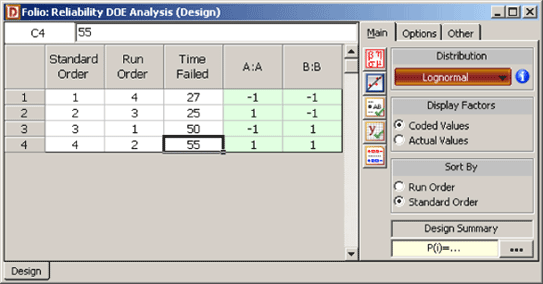
To illustrate the use of MLE in R-DOE analysis, consider the case where the life of a product is thought to be affected by two factors, [math]\displaystyle{ A\,\! }[/math] and [math]\displaystyle{ B\,\! }[/math]. The failure of the product has been found to follow the lognormal distribution. The analyst decides to run an R-DOE analysis using a single replicate of the [math]\displaystyle{ {2}^{2}\,\! }[/math] design. Previous studies indicate that the interaction between [math]\displaystyle{ A\,\! }[/math] and [math]\displaystyle{ B\,\! }[/math] does not affect the life of the product. The design for this experiment can be set up in DOE++ as shown in the following figure.
The resulting experiment design and the corresponding times-to-failure data obtained are shown next. Note that, although the life data set contains complete data and regression techniques are applicable, calculations are shown using MLE. DOE ++ uses MLE for all R-DOE analysis calculations.
Because the purpose of the experiment is to study two factors without considering their interaction, the applicable model for the lognormally distributed response data is:
- [math]\displaystyle{ \mu _{i}^{\prime }={{\beta }_{0}}+{{\beta }_{1}}{{x}_{i1}}+{{\beta }_{2}}{{x}_{i2}}\,\! }[/math]
where [math]\displaystyle{ \mu _{i}^{\prime }\,\! }[/math] is the mean of the natural logarithm of the times-to-failure at the [math]\displaystyle{ i\,\! }[/math]th treatment combination ([math]\displaystyle{ i=1,2,3,4\,\! }[/math]), [math]\displaystyle{ {{\beta }_{1}}\,\! }[/math] is the effect coefficient for factor [math]\displaystyle{ A\,\! }[/math] and [math]\displaystyle{ {{\beta }_{2}}\,\! }[/math] is the effect coefficient for factor [math]\displaystyle{ B\,\! }[/math]. The analysis for this case is carried out in DOE++ by removing the interaction [math]\displaystyle{ AB\,\! }[/math].
The following hypotheses need to be tested in this example:
- 1) [math]\displaystyle{ {{H}_{0}}:{{\beta }_{1}}=0\,\! }[/math]
- [math]\displaystyle{ {{H}_{1}}:{{\beta }_{1}}\ne 0\,\! }[/math]
This test investigates the main effect of factor [math]\displaystyle{ A\,\! }[/math]. The statistic for this test is:
- [math]\displaystyle{ L{{R}_{A}}=-2\ln \frac{{{L}_{\tilde{\ }A}}}{L}\,\! }[/math]
where [math]\displaystyle{ L\,\! }[/math] represents the value of the likelihood function when all coefficients are included in the model and [math]\displaystyle{ {{L}_{\tilde{\ }A}}\,\! }[/math] represents the value of the likelihood function when all coefficients except [math]\displaystyle{ {{\beta }_{1}}\,\! }[/math] are included in the model.
- 2) [math]\displaystyle{ {{H}_{0}}:{{\beta }_{2}}=0\,\! }[/math]
- [math]\displaystyle{ {{H}_{1}}:{{\beta }_{2}}\ne 0\,\! }[/math]
This test investigates the main effect of factor [math]\displaystyle{ B\,\! }[/math]. The statistic for this test is:
- [math]\displaystyle{ L{{R}_{B}}=-2\ln \frac{{{L}_{\tilde{\ }B}}}{L}\,\! }[/math]
where [math]\displaystyle{ L\,\! }[/math] represents the value of the likelihood function when all coefficients are included in the model and [math]\displaystyle{ {{L}_{\tilde{\ }B}}\,\! }[/math] represents the value of the likelihood function when all coefficients except [math]\displaystyle{ {{\beta }_{2}}\,\! }[/math] are included in the model.
To calculate the test statistics, the maximum likelihood estimates of the parameters must be known. The estimates are obtained next.
MLE Estimates
Since the life data for the present experiment are complete and follow the lognormal distribution, the likelihood function can be written as:
- [math]\displaystyle{ L=\underset{i=1}{\overset{4}{\mathop \prod }}\,\left[ \frac{1}{{{t}_{i}}{\sigma }'\sqrt{2\pi }}{{e}^{-\frac{1}{2}{{\left( \frac{\ln ({{t}_{i}})-\mu _{i}^{\prime }}{{{\sigma }'}} \right)}^{2}}}} \right]\,\! }[/math]
Substituting [math]\displaystyle{ \mu _{i}^{\prime }\,\! }[/math] from the applicable model for the lognormally distributed response data, the likelihood function is:
- [math]\displaystyle{ L=\underset{i=1}{\overset{4}{\mathop \prod }}\,\left[ \frac{1}{{{t}_{i}}{\sigma }'\sqrt{2\pi }}{{e}^{-\frac{1}{2}{{\left( \frac{\ln ({{t}_{i}})-({{\beta }_{0}}+{{\beta }_{1}}{{x}_{i1}}+{{\beta }_{2}}{{x}_{i2}})}{{{\sigma }'}} \right)}^{2}}}} \right]\,\! }[/math]
Then the log-likelihood function is:
- [math]\displaystyle{ \begin{align} \Lambda ({\sigma }',{{\beta }_{0}},{{\beta }_{1}},{{\beta }_{2}})= & \ln (L) \\ = & \underset{i=1}{\overset{4}{\mathop \sum }}\,\ln \left[ \frac{1}{{{t}_{i}}{\sigma }'\sqrt{2\pi }}{{e}^{-\frac{1}{2}{{\left( \frac{\ln ({{t}_{i}})-({{\beta }_{0}}+{{\beta }_{1}}{{x}_{i1}}+{{\beta }_{2}}{{x}_{i2}})}{{{\sigma }'}} \right)}^{2}}}} \right] \\ = & \ln \left[ \frac{1}{{{t}_{1}}{{t}_{2}}{{t}_{3}}{{t}_{4}}{{({\sigma }'\sqrt{2\pi })}^{4}}} \right]+ \\ & \left[ -\frac{1}{2}\underset{i=1}{\overset{4}{\mathop \sum }}\,{{\left( \frac{\ln ({{t}_{i}})-({{\beta }_{0}}+{{\beta }_{1}}{{x}_{i1}}+{{\beta }_{2}}{{x}_{i2}})}{{{\sigma }'}} \right)}^{2}} \right] \\ = & -[\ln ({{t}_{1}}{{t}_{2}}{{t}_{3}}{{t}_{4}})+4\ln ({\sigma }')+2\ln (2\pi )]+ \\ & \left[ -\frac{1}{2}\underset{i=1}{\overset{4}{\mathop \sum }}\,{{\left( \frac{\ln ({{t}_{i}})-({{\beta }_{0}}+{{\beta }_{1}}{{x}_{i1}}+{{\beta }_{2}}{{x}_{i2}})}{{{\sigma }'}} \right)}^{2}} \right] \end{align}\,\! }[/math]
To obtain the MLE estimates of the parameters, [math]\displaystyle{ {\sigma }',{{\beta }_{0}},{{\beta }_{1}}\,\! }[/math] and [math]\displaystyle{ {{\beta }_{2}}\,\! }[/math], the log-likelihood function must be differentiated with respect to these parameters:
- [math]\displaystyle{ \begin{align} \frac{\partial \Lambda }{\partial {\sigma }'}= & -\frac{4}{{{\sigma }'}}+\frac{1}{{{({\sigma }')}^{3}}}\underset{i=1}{\overset{4}{\mathop \sum }}\,{{[\ln ({{t}_{i}})-({{\beta }_{0}}+{{\beta }_{1}}{{x}_{i1}}+{{\beta }_{2}}{{x}_{i2}})]}^{2}} \\ \frac{\partial \Lambda }{\partial {{\beta }_{0}}}= & \frac{1}{{{({\sigma }')}^{2}}}\underset{i=1}{\overset{4}{\mathop \sum }}\,[\ln ({{t}_{i}})-({{\beta }_{0}}+{{\beta }_{1}}{{x}_{i1}}+{{\beta }_{2}}{{x}_{i2}})] \\ \frac{\partial \Lambda }{\partial {{\beta }_{1}}}= & \frac{1}{{{({\sigma }')}^{2}}}\underset{i=1}{\overset{4}{\mathop \sum }}\,{{x}_{i1}}[\ln ({{t}_{i}})-({{\beta }_{0}}+{{\beta }_{1}}{{x}_{i1}}+{{\beta }_{2}}{{x}_{i2}})] \\ \frac{\partial \Lambda }{\partial {{\beta }_{2}}}= & \frac{1}{{{({\sigma }')}^{2}}}\underset{i=1}{\overset{4}{\mathop \sum }}\,{{x}_{i2}}[\ln ({{t}_{i}})-({{\beta }_{0}}+{{\beta }_{1}}{{x}_{i1}}+{{\beta }_{2}}{{x}_{i2}})] \end{align}\,\! }[/math]
Equating the [math]\displaystyle{ \partial \Lambda /\partial {{\theta }_{i}}\,\! }[/math] terms to zero returns the required estimates. The coefficients [math]\displaystyle{ {{\hat{\beta }}_{0}}\,\! }[/math], [math]\displaystyle{ {{\hat{\beta }}_{1}}\,\! }[/math] and [math]\displaystyle{ {{\hat{\beta }}_{2}}\,\! }[/math] are obtained first as these are required to estimate [math]\displaystyle{ {{\hat{\sigma }}^{\prime }}\,\! }[/math]. Setting [math]\displaystyle{ \partial \Lambda /\partial {{\beta }_{0}}=0\,\! }[/math]:
- [math]\displaystyle{ \underset{i=1}{\overset{4}{\mathop \sum }}\,[\ln ({{t}_{i}})-({{\beta }_{0}}+{{\beta }_{1}}{{x}_{i1}}+{{\beta }_{2}}{{x}_{i2}})]=0\,\! }[/math]
Substituting the values of [math]\displaystyle{ {{t}_{i}}\,\! }[/math], [math]\displaystyle{ {{x}_{i1}}\,\! }[/math] and [math]\displaystyle{ {{x}_{i2}}\,\! }[/math] from the figure above and simplifying:
- [math]\displaystyle{ \ln {{t}_{1}}+\ln {{t}_{2}}+\ln {{t}_{3}}+\ln {{t}_{4}}-4{{\beta }_{0}}=0\,\! }[/math]
Thus:
- [math]\displaystyle{ \begin{align} {{{\hat{\beta }}}_{0}}= & \frac{1}{4}(\ln {{t}_{1}}+\ln {{t}_{2}}+\ln {{t}_{3}}+\ln {{t}_{4}}) \\ = & \frac{1}{4}(3.2958+3.2189+3.912+4.0073) \\ = & 3.6085 \end{align}\,\! }[/math]
Setting [math]\displaystyle{ \partial \Lambda /\partial {{\beta }_{1}}=0\,\! }[/math]:
- [math]\displaystyle{ {{x}_{i1}}\ln {{t}_{1}}+{{x}_{i1}}\ln {{t}_{2}}+{{x}_{i1}}\ln {{t}_{3}}+{{x}_{i1}}\ln {{t}_{4}}-4{{\beta }_{1}}=0\,\! }[/math]
Thus:
- [math]\displaystyle{ \begin{align} {{{\hat{\beta }}}_{1}}= & \frac{1}{4}(-\ln {{t}_{1}}+\ln {{t}_{2}}-\ln {{t}_{3}}+\ln {{t}_{4}}) \\ = & \frac{1}{4}(-3.2958+3.2189-3.912+4.0073) \\ = & 0.0046 \end{align}\,\! }[/math]
Setting [math]\displaystyle{ \partial \Lambda /\partial {{\beta }_{2}}=0\,\! }[/math]:
- [math]\displaystyle{ {{x}_{i2}}\ln {{t}_{1}}+{{x}_{i2}}\ln {{t}_{2}}+{{x}_{i3}}\ln {{t}_{3}}+{{x}_{i4}}\ln {{t}_{4}}-4{{\beta }_{2}}=0\,\! }[/math]
Thus:
- [math]\displaystyle{ \begin{align} {{{\hat{\beta }}}_{2}}= & \frac{1}{4}(-\ln {{t}_{1}}-\ln {{t}_{2}}+\ln {{t}_{3}}+\ln {{t}_{4}}) \\ = & \frac{1}{4}(-3.2958-3.2189+3.912+4.0073) \\ = & 0.3512 \end{align}\,\! }[/math]
Knowing [math]\displaystyle{ {{\hat{\beta }}_{0}},{{\hat{\beta }}_{1}}\,\! }[/math] and [math]\displaystyle{ {{\hat{\beta }}_{2}}\,\! }[/math], [math]\displaystyle{ {{\hat{\sigma }}^{\prime }}\,\! }[/math] can now be obtained. Setting [math]\displaystyle{ \partial \Lambda /\partial {\sigma }'=0\,\! }[/math]:
- [math]\displaystyle{ -\frac{4}{{{\sigma }'}}+\frac{1}{{{({\sigma }')}^{3}}}\underset{i=1}{\overset{4}{\mathop \sum }}\,{{[\ln ({{t}_{i}})-(3.6085+0.0046{{x}_{i1}}+0.3512{{x}_{i2}})]}^{2}}=0\,\! }[/math]
Thus:
- [math]\displaystyle{ \begin{align} {{{\hat{\sigma }}}^{\prime }}= & \frac{1}{2}\sqrt{\underset{i=1}{\overset{4}{\mathop \sum }}\,{{[\ln ({{t}_{i}})-(3.6085+0.0046{{x}_{i1}}+0.3512{{x}_{i2}})]}^{2}}} \\ = & 0.043 \end{align}\,\! }[/math]
Once the estimates have been calculated, the likelihood ratio test can be carried out for the two factors.
Likelihood Ratio Test
The likelihood ratio test for factor [math]\displaystyle{ A\,\! }[/math] is conducted by using the likelihood value corresponding to the full model and the likelihood value when [math]\displaystyle{ A\,\! }[/math] is not included in the model. The likelihood value corresponding to the full model (in this case [math]\displaystyle{ \mu _{i}^{\prime }={{\beta }_{0}}+{{\beta }_{1}}{{x}_{i1}}+{{\beta }_{2}}{{x}_{i2}}\,\! }[/math]) is:
- [math]\displaystyle{ \begin{align} L= & \underset{i=1}{\overset{4}{\mathop \prod }}\,\left[ \frac{1}{{{t}_{i}}{{{\hat{\sigma }}}^{\prime }}\sqrt{2\pi }}{{e}^{-\frac{1}{2}{{\left( \frac{\ln ({{t}_{i}})-({{{\hat{\beta }}}_{0}}+{{{\hat{\beta }}}_{1}}{{x}_{i1}}+{{{\hat{\beta }}}_{2}}{{x}_{i2}})}{{{{\hat{\sigma }}}^{\prime }}} \right)}^{2}}}} \right] \\ = & 0.000537311 \end{align}\,\! }[/math]
The corresponding logarithmic value is [math]\displaystyle{ \ln (L)=\ln (0.000537311)=-7.529\,\! }[/math].
The likelihood value for the reduced model that does not contain factor [math]\displaystyle{ A\,\! }[/math] (in this case [math]\displaystyle{ \mu _{i}^{\prime }={{\beta }_{0}}+{{\beta }_{2}}{{x}_{i2}}\,\! }[/math]) is:
- [math]\displaystyle{ \begin{align} {{L}_{\tilde{\ }A}}= & \underset{i=1}{\overset{4}{\mathop \prod }}\,\left[ \frac{1}{{{t}_{i}}{{{\hat{\sigma }}}^{\prime }}\sqrt{2\pi }}{{e}^{-\frac{1}{2}{{\left( \frac{\ln ({{t}_{i}})-({{{\hat{\beta }}}_{0}}+{{{\hat{\beta }}}_{2}}{{x}_{i2}})}{{{{\hat{\sigma }}}^{\prime }}} \right)}^{2}}}} \right] \\ = & 0.000525337 \end{align}\,\! }[/math]
The corresponding logarithmic value is [math]\displaystyle{ \ln ({{L}_{\tilde{\ }A}})=\ln (0.000525337)=-7.552\,\! }[/math].
Therefore, the likelihood ratio to test the significance of factor [math]\displaystyle{ A\,\! }[/math] is:
- [math]\displaystyle{ \begin{align} L{{R}_{A}}= & -2\ln \frac{{{L}_{\tilde{\ }A}}}{L} \\ = & -2\ln \frac{0.000525337}{0.000537311} \\ = & 0.0451 \end{align}\,\! }[/math]
The [math]\displaystyle{ p\,\! }[/math] value corresponding to [math]\displaystyle{ L{{R}_{A}}\,\! }[/math] is:
- [math]\displaystyle{ \begin{align} p\text{ }value= & 1-P(\chi _{1}^{2}\lt L{{R}_{A}}) \\ = & 1-0.1682 \\ = & 0.8318 \end{align}\,\! }[/math]
Assuming that the desired significance level for the present experiment is 0.1, since [math]\displaystyle{ p\,\! }[/math] [math]\displaystyle{ value\gt 0.1\,\! }[/math], [math]\displaystyle{ {{H}_{0}}:{{\beta }_{1}}=0\,\! }[/math] cannot be rejected and it can be concluded that factor [math]\displaystyle{ A\,\! }[/math] does not affect the life of the product.
The likelihood ratio to test factor [math]\displaystyle{ B\,\! }[/math] can be calculated in a similar way as shown next:
- [math]\displaystyle{ \begin{align} L{{R}_{B}}= & -2\ln \frac{{{L}_{\tilde{\ }B}}}{L} \\ = & -2\ln \frac{1.17995E-07}{0.000537311} \\ = & 16.8475 \end{align}\,\! }[/math]
The [math]\displaystyle{ p\,\! }[/math] value corresponding to [math]\displaystyle{ L{{R}_{B}}\,\! }[/math] is:
- [math]\displaystyle{ \begin{align} p\text{ }value= & 1-P(\chi _{1}^{2}\lt L{{R}_{B}}) \\ = & 1-0.99996 \\ = & 0.00004 \end{align}\,\! }[/math]
Since [math]\displaystyle{ p\,\! }[/math] [math]\displaystyle{ value\lt 0.1\,\! }[/math], [math]\displaystyle{ {{H}_{0}}:{{\beta }_{2}}=0\,\! }[/math] is rejected and it is concluded that factor [math]\displaystyle{ B\,\! }[/math] affects the life of the product. The previous calculation results are displayed as the Likelihood Ratio Test Table in the results obtained from DOE++ as shown in the figure below.

Fisher Matrix Bounds on Parameters
In general, the MLE estimates of the parameters are asymptotically normal. This means that for large sample sizes the distribution of the estimates from the same population would be very close to the normal distribution [Meeker and Escobar]. If [math]\displaystyle{ \hat{\theta }\,\! }[/math] is the MLE estimate of any parameter, [math]\displaystyle{ \theta \,\! }[/math], then the ([math]\displaystyle{ 1-\alpha \,\! }[/math])% two-sided confidence bounds on the parameter are:
- [math]\displaystyle{ \hat{\theta }-{{z}_{\alpha /2}}\cdot \sqrt{Var(\hat{\theta })}\lt \theta \lt \hat{\theta }+{{z}_{\alpha /2}}\cdot \sqrt{Var(\hat{\theta })}\,\! }[/math]
where [math]\displaystyle{ Var(\hat{\theta })\,\! }[/math] represents the variance of [math]\displaystyle{ \hat{\theta }\,\! }[/math] and [math]\displaystyle{ {{z}_{\alpha /2}}\,\! }[/math] is the critical value corresponding to a significance level of [math]\displaystyle{ \alpha /2\,\! }[/math] on the standard normal distribution. The variance of the parameter, [math]\displaystyle{ Var(\hat{\theta })\,\! }[/math], is obtained using the Fisher information matrix. For [math]\displaystyle{ k\,\! }[/math] parameters, the Fisher information matrix is obtained from the log-likelihood function [math]\displaystyle{ \Lambda \,\! }[/math] as follows:
- [math]\displaystyle{ F=\left[ \begin{matrix} -\frac{{{\partial }^{2}}\Lambda }{\partial \theta _{1}^{2}} & -\frac{{{\partial }^{2}}\Lambda }{\partial {{\theta }_{1}}\partial {{\theta }_{2}}} & ... & -\frac{{{\partial }^{2}}\Lambda }{\partial {{\theta }_{1}}\partial {{\theta }_{k}}} \\ -\frac{{{\partial }^{2}}\Lambda }{\partial {{\theta }_{1}}\partial {{\theta }_{2}}} & -\frac{{{\partial }^{2}}\Lambda }{\partial \theta _{2}^{2}} & ... & -\frac{{{\partial }^{2}}\Lambda }{\partial {{\theta }_{2}}\partial {{\theta }_{k}}} \\ . & . & ... & . \\ . & . & ... & . \\ -\frac{{{\partial }^{2}}\Lambda }{\partial {{\theta }_{1}}\partial {{\theta }_{k}}} & . & ... & -\frac{{{\partial }^{2}}\Lambda }{\partial \theta _{k}^{2}} \\ \end{matrix} \right]\,\! }[/math]
The variance-covariance matrix is obtained by inverting the Fisher matrix [math]\displaystyle{ F\,\! }[/math]:
- [math]\displaystyle{ \left[ \begin{matrix} Var({{{\hat{\theta }}}_{1}}) & Cov({{{\hat{\theta }}}_{1}},{{{\hat{\theta }}}_{2}}) & ... & {} \\ Cov({{{\hat{\theta }}}_{1}},{{{\hat{\theta }}}_{2}}) & Var({{{\hat{\theta }}}_{2}}) & ... & {} \\ . & . & ... & {} \\ . & . & ... & {} \\ Cov({{{\hat{\theta }}}_{1}},{{{\hat{\theta }}}_{k}}) & . & ... & Var({{{\hat{\theta }}}_{k}}) \\ \end{matrix} \right]=\,\! }[/math]
- [math]\displaystyle{ {{\left[ \begin{matrix} -\frac{{{\partial }^{2}}\Lambda }{\partial \theta _{1}^{2}} & -\frac{{{\partial }^{2}}\Lambda }{\partial {{\theta }_{1}}\partial {{\theta }_{2}}} & ... & {} \\ -\frac{{{\partial }^{2}}\Lambda }{\partial {{\theta }_{1}}\partial {{\theta }_{2}}} & -\frac{{{\partial }^{2}}\Lambda }{\partial \theta _{2}^{2}} & ... & {} \\ . & . & ... & {} \\ . & . & ... & {} \\ -\frac{{{\partial }^{2}}\Lambda }{\partial {{\theta }_{1}}\partial {{\theta }_{k}}} & . & ... & -\frac{{{\partial }^{2}}\Lambda }{\partial \theta _{k}^{2}} \\ \end{matrix} \right]}^{-1}}\,\! }[/math]
Once the variance-covariance matrix is known the variance of any parameter can be obtained from the diagonal elements of the matrix. Note that if a parameter, [math]\displaystyle{ \theta \,\! }[/math], can take only positive values, it is assumed that the [math]\displaystyle{ \ln (\hat{\theta })\,\! }[/math] follows the normal distribution [Meeker and Escobar]. The bounds on the parameter in this case are:
- [math]\displaystyle{ CI\text{ }on\text{ }\ln (\hat{\theta })=\ln (\hat{\theta })\pm {{z}_{\alpha /2}}\sqrt{Var(\ln (\hat{\theta }))}\,\! }[/math]
Using [math]\displaystyle{ Var[f(\hat{\theta })]={{(\partial f/\partial \theta )}^{2}}\cdot Var(\hat{\theta })\,\! }[/math] we get [math]\displaystyle{ Var(\ln (\hat{\theta }))={{(1/\hat{\theta })}^{2}}Var(\hat{\theta })\,\! }[/math]. Substituting this value we have:
- [math]\displaystyle{ \begin{align} CI\text{ }on\text{ }\ln (\hat{\theta })= & \ln (\hat{\theta })\pm {{z}_{\alpha /2}}\sqrt{{{(1/\hat{\theta })}^{2}}Var(\hat{\theta })} \\ = & \ln (\hat{\theta })\pm ({{z}_{\alpha /2}}/\hat{\theta })\sqrt{Var(\hat{\theta })} \\ or\text{ }CI\text{ }on\text{ }\hat{\theta }= & \exp [\ln (\hat{\theta })\pm ({{z}_{\alpha /2}}/\hat{\theta })\sqrt{Var(\hat{\theta })}] \\ = & \hat{\theta }\cdot \exp [\pm ({{z}_{\alpha /2}}/\hat{\theta })\sqrt{Var(\hat{\theta })}] \end{align}\,\! }[/math]
Knowing [math]\displaystyle{ Var(\hat{\theta })\,\! }[/math] from the variance-covariance matrix, the confidence bounds on [math]\displaystyle{ \hat{\theta }\,\! }[/math] can then be determined.
Example
Continuing with the example, the confidence bounds on the MLE estimates of the parameters [math]\displaystyle{ {{\beta }_{0}}\,\! }[/math], [math]\displaystyle{ {{\beta }_{1}}\,\! }[/math], [math]\displaystyle{ {{\beta }_{2}}\,\! }[/math] and [math]\displaystyle{ {\sigma }'\,\! }[/math] can now be obtained. The Fisher information matrix for the example is:
- [math]\displaystyle{ \begin{align} F= & \left[ \begin{matrix} -\frac{{{\partial }^{2}}\Lambda }{\partial \beta _{0}^{2}} & -\frac{{{\partial }^{2}}\Lambda }{\partial {{\beta }_{0}}\partial {{\beta }_{1}}} & -\frac{{{\partial }^{2}}\Lambda }{\partial {{\beta }_{0}}\partial {{\beta }_{2}}} & -\frac{{{\partial }^{2}}\Lambda }{\partial {{\beta }_{0}}\partial {\sigma }'} \\ {} & -\frac{{{\partial }^{2}}\Lambda }{\partial \beta _{1}^{2}} & -\frac{{{\partial }^{2}}\Lambda }{\partial {{\beta }_{1}}\partial {{\beta }_{2}}} & -\frac{{{\partial }^{2}}\Lambda }{\partial {{\beta }_{1}}\partial {\sigma }'} \\ {} & {} & -\frac{{{\partial }^{2}}\Lambda }{\partial \beta _{2}^{2}} & -\frac{{{\partial }^{2}}\Lambda }{\partial {{\beta }_{2}}\partial {\sigma }'} \\ sym. & {} & {} & -\frac{{{\partial }^{2}}\Lambda }{\partial {{\sigma }^{\prime 2}}} \\ \end{matrix} \right] \\ = & \left[ \begin{matrix} \tfrac{4}{{{\sigma }^{\prime 2}}} & \tfrac{1}{{{\sigma }^{\prime 2}}}\underset{i=1}{\overset{4}{\mathop{\sum }}}\,{{x}_{i1}} & \tfrac{1}{{{\sigma }^{\prime 2}}}\underset{i=1}{\overset{4}{\mathop{\sum }}}\,{{x}_{i2}} & \tfrac{2}{{{\sigma }^{\prime 3}}}[\underset{i=1}{\overset{4}{\mathop{\sum }}}\,(\ln {{t}_{i}}-\mu _{i}^{\prime })] \\ {} & \tfrac{1}{{{\sigma }^{\prime 2}}}\underset{i=1}{\overset{4}{\mathop{\sum }}}\,x_{i1}^{2} & \tfrac{1}{{{\sigma }^{\prime 2}}}\underset{i=1}{\overset{4}{\mathop{\sum }}}\,{{x}_{i1}}{{x}_{i2}} & \tfrac{2}{{{\sigma }^{\prime 3}}}[\underset{i=1}{\overset{4}{\mathop{\sum }}}\,{{x}_{i1}}\cdot (\ln {{t}_{i}}-\mu _{i}^{\prime })] \\ {} & {} & \tfrac{1}{{{\sigma }^{\prime 2}}}\underset{i=1}{\overset{4}{\mathop{\sum }}}\,x_{i2}^{2} & \tfrac{2}{{{\sigma }^{\prime 3}}}[\underset{i=1}{\overset{4}{\mathop{\sum }}}\,{{x}_{i2}}\cdot (\ln {{t}_{i}}-\mu _{i}^{\prime })] \\ sym. & {} & {} & \tfrac{4}{{{\sigma }^{\prime 2}}}+\tfrac{(-3)}{{{\sigma }^{\prime 4}}}\underset{i=1}{\overset{4}{\mathop{\sum }}}\,{{(\ln {{t}_{i}}-\mu _{i}^{\prime })}^{2}}] \\ \end{matrix} \right] \\ = & \left[ \begin{matrix} 2165.6741 & 0 & 0 & -1.1195E-11 \\ {} & 2165.6741 & 0 & -1.1195E-11 \\ {} & {} & 2165.6741 & -3.358E-11 \\ sym. & {} & {} & 4330.8227 \\ \end{matrix} \right] \end{align}\,\! }[/math]
The variance-covariance matrix can be obtained by taking the inverse of the Fisher matrix [math]\displaystyle{ F\,\! }[/math]:
- [math]\displaystyle{ \left[ \begin{matrix} Var({{{\hat{\beta }}}_{0}}) & Cov({{{\hat{\beta }}}_{0}},{{{\hat{\beta }}}_{1}}) & Cov({{{\hat{\beta }}}_{0}},{{{\hat{\beta }}}_{2}}) & Cov({{{\hat{\beta }}}_{0}},{{{\hat{\sigma }}}^{\prime }}) \\ {} & Var({{{\hat{\beta }}}_{1}}) & Cov({{{\hat{\beta }}}_{1}},{{{\hat{\beta }}}_{2}}) & Cov({{{\hat{\beta }}}_{0}},{{{\hat{\sigma }}}^{\prime }}) \\ {} & {} & Var({{{\hat{\beta }}}_{2}}) & Cov({{{\hat{\beta }}}_{0}},{{{\hat{\sigma }}}^{\prime }}) \\ sym. & {} & {} & Var({{{\hat{\sigma }}}^{\prime }}) \\ \end{matrix} \right]={{F}^{-1}}\,\! }[/math]
Inverting [math]\displaystyle{ F\,\! }[/math] returns the following matrix:
- [math]\displaystyle{ {{F}^{-1}}=\left[ \begin{matrix} 4.617E-4 & 0 & 0 & 0 \\ {} & 4.617E-4 & 0 & 0 \\ {} & {} & 4.617E-4 & 0 \\ sym. & {} & {} & 2.309E-4 \\ \end{matrix} \right]\,\! }[/math]
Therefore, the variance of the parameter estimates are:
- [math]\displaystyle{ \begin{align} Var({{{\hat{\beta }}}_{0}})= & 4.617E-4 \\ Var({{{\hat{\beta }}}_{1}})= & 4.617E-4 \\ Var({{{\hat{\beta }}}_{2}})= & 4.617E-4 \\ Var({{{\hat{\sigma }}}^{\prime }})= & 2.309E-4 \end{align}\,\! }[/math]
Knowing the variance, the confidence bounds on the parameters can be calculated. For example, the 90% bounds ([math]\displaystyle{ \alpha =0.1\,\! }[/math]) on [math]\displaystyle{ {{\hat{\beta }}_{2}}\,\! }[/math] can be calculated as shown next:
- [math]\displaystyle{ \begin{align} CI= & {{{\hat{\beta }}}_{2}}\pm {{z}_{\alpha /2}}\cdot \sqrt{Var({{{\hat{\beta }}}_{2}})} \\ = & {{{\hat{\beta }}}_{2}}\pm {{z}_{0.05}}\cdot \sqrt{Var({{{\hat{\beta }}}_{2}})} \\ = & 0.3512\pm 1.645\cdot \sqrt{4.617E-4} \\ = & 0.3512\pm 0.0354 \\ = & 0.3158\text{ }and\text{ }0.3866 \end{align}\,\! }[/math]
The 90% bounds on [math]\displaystyle{ {\sigma }'\,\! }[/math] are (considering that [math]\displaystyle{ {\sigma }'\,\! }[/math] can only take positive values):
- [math]\displaystyle{ \begin{align} CI= & {{{\hat{\sigma }}}^{\prime }}\cdot \exp [\pm ({{z}_{0.05}}/{{{\hat{\sigma }}}^{\prime }})\sqrt{Var({{{\hat{\sigma }}}^{\prime }})}] \\ = & 0.043\cdot \exp [\pm (1.645/0.043)\sqrt{2.309E-4}] \\ = & 0.024\text{ }and\text{ }0.077 \end{align}\,\! }[/math]
The standard error for the parameters can be obtained by taking the positive square root of the variance. For example, the standard error for [math]\displaystyle{ {{\hat{\beta }}_{1}}\,\! }[/math] is:
- [math]\displaystyle{ \begin{align} se({{{\hat{\beta }}}_{1}})= & \sqrt{Var({{{\hat{\beta }}}_{1}})} \\ = & \sqrt{4.617E-4} \\ = & 0.0215 \end{align}\,\! }[/math]
The [math]\displaystyle{ z\,\! }[/math] statistic for [math]\displaystyle{ {{\hat{\beta }}_{1}}\,\! }[/math] is:
- [math]\displaystyle{ \begin{align} {{z}_{0}}= & \frac{{{{\hat{\beta }}}_{1}}}{se({{{\hat{\beta }}}_{1}})} \\ = & \frac{0.0046}{0.0215} \\ = & 0.21 \end{align}\,\! }[/math]
The [math]\displaystyle{ p\,\! }[/math] value corresponding to this statistic based on the standard normal distribution is:
- [math]\displaystyle{ \begin{align} p\text{ }value= & 2\cdot (1-P(Z\le |{{z}_{0}}|) \\ = & 2\cdot (1-0.58435) \\ = & 0.8313 \end{align}\,\! }[/math]
The previous calculation results are displayed as MLE Information in the results obtained from DOE++ as shown in the following figure. In the figure, the Effect corresponding to each factor is simply twice the MLE estimate of the coefficient for that factor. Generally, the [math]\displaystyle{ p\,\! }[/math] value corresponding to any coefficient in the MLE Information table should match the value obtained from the likelihood ratio test (displayed in the Likelihood Ratio Test table of the figure below). If the sample size is not large enough, as in the case of the present example, a difference may be seen in the two values. In such cases, the [math]\displaystyle{ p\,\! }[/math] value from the likelihood ratio test should be given preference. For the present example, the [math]\displaystyle{ p\,\! }[/math] value of 0.8318 for [math]\displaystyle{ {{\hat{\beta }}_{1}}\,\! }[/math], obtained from the likelihood ratio test, would be preferred to the [math]\displaystyle{ p\,\! }[/math] value of 0.8313 displayed under MLE information. For details see [Meeker and Escobar].

R-DOE Analysis of Data Following the Weibull Distribution
The probability density function for the 2-parameter Weibull distribution is:
- [math]\displaystyle{ f(T)=\frac{\beta }{\eta }{{\left( \frac{T}{\eta } \right)}^{\beta -1}}\exp \left[ -{{\left( \frac{T}{\eta } \right)}^{\beta }} \right]\,\! }[/math]
where [math]\displaystyle{ \eta \,\! }[/math] is the scale parameter of the Weibull distribution and [math]\displaystyle{ \beta \,\! }[/math] is the shape parameter [Life Data Analysis Reference]. To distinguish the Weibull shape parameter from the effect coefficients, the shape parameter is represented as [math]\displaystyle{ Beta\,\! }[/math] instead of [math]\displaystyle{ \beta \,\! }[/math] in the remaining chapter.
For data following the 2-parameter Weibull distribution, the life characteristic used in R-DOE analysis is the scale parameter, [math]\displaystyle{ \eta \,\! }[/math] [Accelerated Life Testing Reference]. Since [math]\displaystyle{ \eta \,\! }[/math] represents life data that cannot take negative values, a logarithmic transformation is applied to it. The resulting model used in the R-DOE analysis for a two factor experiment with each factor at two levels can be written as follows:
- [math]\displaystyle{ \ln ({{\eta }_{i}})={{\beta }_{0}}+{{\beta }_{1}}{{x}_{i1}}+{{\beta }_{2}}{{x}_{i2}}+{{\beta }_{12}}{{x}_{i1}}{{x}_{i2}}\,\! }[/math]
where:
- [math]\displaystyle{ {{\eta }_{i}}\,\! }[/math] is the value of the scale parameter at the [math]\displaystyle{ i\,\! }[/math]th treatment combination of the two factors
- [math]\displaystyle{ {{x}_{1}}\,\! }[/math] is the indicator variable representing the level of the first factor
- [math]\displaystyle{ {{x}_{2}}\,\! }[/math] is the indicator variable representing the level of the second factor
- [math]\displaystyle{ {{\beta }_{0}}\,\! }[/math] is the intercept term
- [math]\displaystyle{ {{\beta }_{1}}\,\! }[/math] and [math]\displaystyle{ {{\beta }_{2}}\,\! }[/math] are the effect coefficients for the two factors
- and [math]\displaystyle{ {{\beta }_{12}}\,\! }[/math] is the effect coefficient for the interaction of the two factors
The model can be easily expanded to include other factors and their interactions. Note that when any data follows the Weibull distribution, the logarithmic transformation of the data follows the extreme-value distribution, whose probability density function is given as follows:
- [math]\displaystyle{ f(\ln (T))=\frac{1}{{{\sigma }''}}\exp \left[ \frac{\ln (T)-{\mu }''}{{{\sigma }''}}-\exp \left( \frac{\ln (T)-{\mu }''}{{{\sigma }''}} \right) \right]\,\! }[/math]
where the [math]\displaystyle{ T\,\! }[/math]s follow the Weibull distribution, [math]\displaystyle{ {\mu }''\,\! }[/math] is the location parameter of the extreme-value distribution and [math]\displaystyle{ {\sigma }''\,\! }[/math] is the scale parameter of the extreme-value distribution. The two equations given above show that for R-DOE analysis of life data that follows the Weibull distribution, the random error terms, [math]\displaystyle{ {{\epsilon }_{i}}\,\! }[/math], will follow the extreme-value distribution (and not the normal distribution). Hence, regression techniques are not applicable even if the data is complete. Therefore, maximum likelihood estimation has to be used.
Maximum Likelihood Estimation for the Weibull Distribution
The likelihood function for complete data in R-DOE analysis of Weibull distributed life data is:
- [math]\displaystyle{ \begin{align} {{L}_{failures}}= & \underset{i=1}{\overset{{{F}_{e}}}{\mathop{\prod }}}\,f({{t}_{i}},{{\eta }_{i}}) \\ = & \underset{i=1}{\overset{{{F}_{e}}}{\mathop{\prod }}}\,\left[ \frac{Beta}{{{\eta }_{i}}}{{\left( \frac{{{t}_{i}}}{{{\eta }_{i}}} \right)}^{Beta-1}}\exp \left[ -{{\left( \frac{{{t}_{i}}}{{{\eta }_{i}}} \right)}^{Beta}} \right] \right] \end{align}\,\! }[/math]
where:
- [math]\displaystyle{ {{F}_{e}}\,\! }[/math] is the total number of observed times-to-failure
- [math]\displaystyle{ {{\eta }_{i}}\,\! }[/math] is the life characteristic at the [math]\displaystyle{ i\,\! }[/math]th treatment
- and [math]\displaystyle{ {{t}_{i}}\,\! }[/math] is the time of the [math]\displaystyle{ i\,\! }[/math]th failure
For right censored data, the likelihood function is:
- [math]\displaystyle{ {{L}_{suspensions}}=\underset{i=1}{\overset{{{S}_{e}}}{\mathop{\prod }}}\,\left[ \exp \left[ -{{\left( \frac{{{t}_{i}}}{{{\eta }_{i}}} \right)}^{Beta}} \right] \right]\,\! }[/math]
where:
- [math]\displaystyle{ {{S}_{e}}\,\! }[/math] is the total number of observed suspensions
- and [math]\displaystyle{ {{t}_{i}}\,\! }[/math] is the time of [math]\displaystyle{ i\,\! }[/math]th suspension
For interval data, the likelihood function is:
- [math]\displaystyle{ {{L}_{interval}}=\underset{i=1}{\overset{FI}{\mathop{\prod }}}\,\left[ \exp \left[ -{{\left( \frac{t_{i}^{2}}{{{\eta }_{i}}} \right)}^{Beta}} \right]-\exp \left[ -{{\left( \frac{t_{i}^{1}}{{{\eta }_{i}}} \right)}^{Beta}} \right] \right]\,\! }[/math]
where:
- [math]\displaystyle{ FI\,\! }[/math] is the total number of interval data
- [math]\displaystyle{ t_{i}^{1}\,\! }[/math] is the beginning time of the [math]\displaystyle{ i\,\! }[/math]th interval
- and [math]\displaystyle{ t_{i}^{2}\,\! }[/math] is the end time of the [math]\displaystyle{ i\,\! }[/math] th interval
In each of the likelihood functions, [math]\displaystyle{ {{\eta }_{i}}\,\! }[/math] is substituted as:
- [math]\displaystyle{ {{\eta }_{i}}=\exp ({{\beta }_{0}}+{{\beta }_{1}}{{x}_{i1}}+{{\beta }_{2}}{{x}_{i2}}+...)\,\! }[/math]
The complete likelihood function when all types of data (complete, right and left censored) are present is:
- [math]\displaystyle{ L(Beta,{{\beta }_{0}},{{\beta }_{1}}...)={{L}_{failures}}\cdot {{L}_{suspensions}}\cdot {{L}_{interval}}\,\! }[/math]
Then the log-likelihood function is:
- [math]\displaystyle{ \Lambda (Beta,{{\beta }_{0}},{{\beta }_{1}}...)=\ln (L)\,\! }[/math]
The MLE estimates are obtained by solving for parameters [math]\displaystyle{ (Beta,{{\beta }_{0}},{{\beta }_{1}}...)\,\! }[/math] so that:
- [math]\displaystyle{ \begin{align} \frac{\partial \Lambda }{\partial Beta}= & 0 \\ \frac{\partial \Lambda }{\partial {{\beta }_{0}}}= & 0 \\ \frac{\partial \Lambda }{\partial {{\beta }_{1}}}= & 0 \\ & ... \end{align}\,\! }[/math]
Once the estimates are obtained, the significance of any parameter, [math]\displaystyle{ {{\theta }_{i}}\,\! }[/math], can be assessed using the likelihood ratio test. Other results can also be obtained as discussed in Sections MLE for the Lognormal and Fisher Matrix Bounds on Parameters.
R-DOE Analysis of Data Following the Exponential Distribution
The exponential distribution is a special case of the Weibull distribution when the shape parameter [math]\displaystyle{ Beta\,\! }[/math] is equal to 1. Substituting [math]\displaystyle{ Beta=1\,\! }[/math] in the probability density function for the 2-parameter Weibull distribution gives:
- [math]\displaystyle{ \begin{align} f(T)= & \frac{1}{\eta }\exp \left( -\frac{T}{\eta } \right) \\ = & \lambda \exp (-\lambda T) \end{align}\,\! }[/math]
where [math]\displaystyle{ 1/\eta \,\! }[/math] of the Weibull pdf has been replaced by [math]\displaystyle{ \lambda \,\! }[/math]. Parameter [math]\displaystyle{ \lambda \,\! }[/math] is called the failure rate [Life Data Analysis Reference]. Hence, R-DOE analysis for exponentially distributed data can be carried out by substituting [math]\displaystyle{ Beta=1\,\! }[/math] and replacing [math]\displaystyle{ 1/\eta \,\! }[/math] by [math]\displaystyle{ \lambda \,\! }[/math] in the Weibull distribution.
Model Diagnostics
Residual plots can be used to check if the model obtained, based on the MLE estimates, is a good fit to the data. DOE++ uses standardized residuals for R-DOE analyses. If the data follows the lognormal distribution, then standardized residuals are calculated using the following equation:
- [math]\displaystyle{ \begin{align} {{{\hat{e}}}_{i}}= & \frac{\ln ({{t}_{i}})-{{{\hat{\mu }}}_{i}}}{{{{\hat{\sigma }}}^{\prime }}} \\ = & \frac{\ln ({{t}_{i}})-({{{\hat{\beta }}}_{0}}+{{{\hat{\beta }}}_{1}}{{x}_{i1}}+{{{\hat{\beta }}}_{2}}{{x}_{i2}}+...)}{{{{\hat{\sigma }}}^{\prime }}} \end{align}\,\! }[/math]
For the probability plot, the standardized residuals are displayed on a normal probability plot. This is because under the assumed model for the lognormal distribution, the standardized residuals should follow a normal distribution with a mean of 0 and a standard deviation of 1.
For data that follows the Weibull distribution, the standardized residuals are calculated as shown next:
- [math]\displaystyle{ \begin{align} {{{\hat{e}}}_{i}}= & \hat{B}eta[\ln ({{t}_{i}})-\ln ({{{\hat{\eta }}}_{i}})] \\ = & \hat{B}eta[\ln ({{t}_{i}})-({{{\hat{\beta }}}_{0}}+{{{\hat{\beta }}}_{1}}{{x}_{i1}}+{{{\hat{\beta }}}_{2}}{{x}_{i2}}+...)] \end{align}\,\! }[/math]
The probability plot, in this case, is used to check if the residuals follow the extreme-value distribution with a mean of 0. Note that in all residual plots, when an observation, [math]\displaystyle{ {{t}_{i}}\,\! }[/math], is censored the corresponding residual is also censored.
Application Examples
Using R-DOE Analysis to Improve Product Reliability
This example illustrates the use of R-DOE analysis to design reliability into a product. An experiment was carried out to investigate the effect of five factors (each at two levels) on the reliability of fluorescent lights [Taguchi, 1987, p. 930]. The factors, [math]\displaystyle{ A\,\! }[/math] through [math]\displaystyle{ E\,\! }[/math], were studied using a [math]\displaystyle{ 2^{5-2}\,\! }[/math] design (with the defining relations [math]\displaystyle{ D=-AC\,\! }[/math] and [math]\displaystyle{ E=-BC\,\! }[/math]) under the assumption that all interaction effects except [math]\displaystyle{ AB\,\! }[/math] [math]\displaystyle{ (=DE)\,\! }[/math] can be assumed to be inactive. For each treatment, two lights were tested (two replicates) with the readings taken every two days. The experiment was run for 20 days, and if a light had not failed by the 20th day, then it was assumed to be a suspension. The experimental design and the corresponding failure times are shown next.
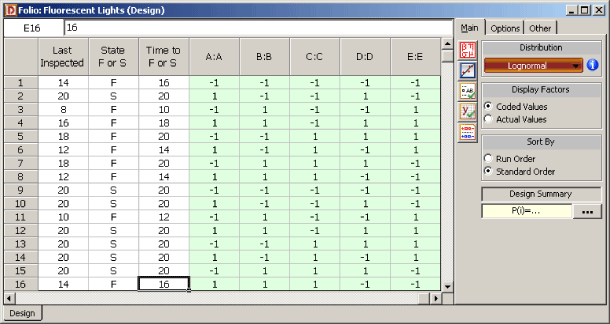
The short duration of the experiment and failure times are probably due to the lights being tested under higher than normal stress levels. The failure of the lights was assumed to follow the lognormal distribution.
The analysis results from DOE++ for this experiment are shown next.
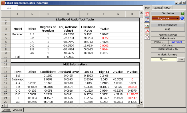
The results are obtained by selecting to use the main effects of the five factors and the interaction [math]\displaystyle{ AB\,\! }[/math] in the analysis. The results show that factors [math]\displaystyle{ B\,\! }[/math], [math]\displaystyle{ D\,\! }[/math] and [math]\displaystyle{ E\,\! }[/math] are active at a significance level of 0.05. The MLE estimates of the effect coefficients corresponding to these factors are [math]\displaystyle{ -0.2015\,\! }[/math], [math]\displaystyle{ 0.2729\,\! }[/math] and [math]\displaystyle{ -0.1527\,\! }[/math], respectively. Based on these coefficients, the best settings for these effects to improve the reliability of the fluorescent lights by maximizing the response (i.e., failure time) are as follows:
- Factor [math]\displaystyle{ B\,\! }[/math] should be set at the lower level of [math]\displaystyle{ -1\,\! }[/math] since its coefficient is negative
- Factor [math]\displaystyle{ D\,\! }[/math] should be set at the higher level of [math]\displaystyle{ 1\,\! }[/math] since its coefficient is positive
- Factor [math]\displaystyle{ E\,\! }[/math] should be set at the lower level of [math]\displaystyle{ -1\,\! }[/math] since its coefficient is negative
Note that, since actual factor levels are not disclosed (presumably for proprietary reasons), predictions beyond the test conditions cannot be carried out in this case.
Using DOE++ with ALTA to Estimate the B10 Life
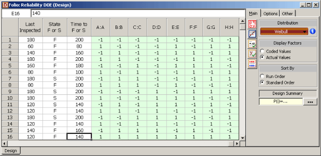
Consider a product whose reliability is thought to be affected by eight potential factors: [math]\displaystyle{ A\,\! }[/math] (temperature), [math]\displaystyle{ B\,\! }[/math] (humidity), [math]\displaystyle{ C\,\! }[/math] (load), [math]\displaystyle{ D\,\! }[/math] (fan-speed), [math]\displaystyle{ E\,\! }[/math] (voltage), [math]\displaystyle{ F\,\! }[/math] (material), [math]\displaystyle{ G\,\! }[/math] (vibration) and [math]\displaystyle{ H\,\! }[/math] (current). Assuming that all interaction effects are absent, a [math]\displaystyle{ 2^{8-4}\,\! }[/math] design is used to investigate the eight factors at two levels. The generators used to obtain the design are [math]\displaystyle{ E=ABC\,\! }[/math], [math]\displaystyle{ F=BCD\,\! }[/math], [math]\displaystyle{ G=ACD\,\! }[/math] and [math]\displaystyle{ H=ABD\,\! }[/math].
Readings for the experiment are taken every 20 time units and the test is terminated at 200 time units. The life of the product is assumed to follow the Weibull distribution. The design and the corresponding life data obtained are shown in the figure below.
The results from DOE++ for this experiment are shown in the figure below.
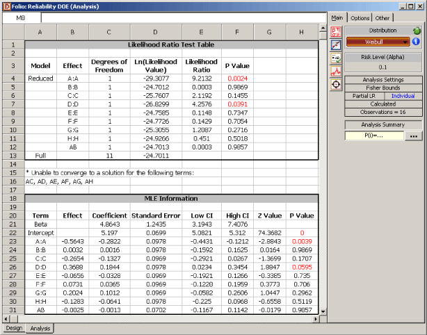
The results show that only factors [math]\displaystyle{ A\,\! }[/math] and [math]\displaystyle{ D\,\! }[/math] are active at a significance level of 0.1.
Assume that, in terms of the actual units, the [math]\displaystyle{ -1\,\! }[/math] level of factor [math]\displaystyle{ A\,\! }[/math] corresponds to a temperature of 333 [math]\displaystyle{ K\,\! }[/math] and the [math]\displaystyle{ +1\,\! }[/math] level corresponds to a temperature of 383 [math]\displaystyle{ K\,\! }[/math]. Similarly, assume that the two levels of factor [math]\displaystyle{ D\,\! }[/math] are 1000 [math]\displaystyle{ rpm\,\! }[/math] and 2000 [math]\displaystyle{ rpm\,\! }[/math] respectively. From the MLE estimates of the effect coefficients it can be noted that to improve reliability (by maximizing the response) factors [math]\displaystyle{ A\,\! }[/math] and [math]\displaystyle{ D\,\! }[/math] should be set as follows:
- Factor [math]\displaystyle{ A\,\! }[/math] should be set at the lower level of 333 [math]\displaystyle{ K\,\! }[/math] since its coefficient is negative
- Factor [math]\displaystyle{ D\,\! }[/math] should be set at the higher level of 2000 [math]\displaystyle{ rpm\,\! }[/math] since its coefficient is positive
Now assume that the use conditions for the product for the significant factors, [math]\displaystyle{ A\,\! }[/math] and [math]\displaystyle{ D\,\! }[/math], are a temperature of 298 [math]\displaystyle{ K\,\! }[/math] and a fan-speed of 3000 [math]\displaystyle{ rpm,\,\! }[/math] respectively. The analysis can be taken a step further to obtain an estimate of the reliability of the product at the use conditions using ReliaSoft's ALTA software. The data is entered into ALTA as shown in the figure below.
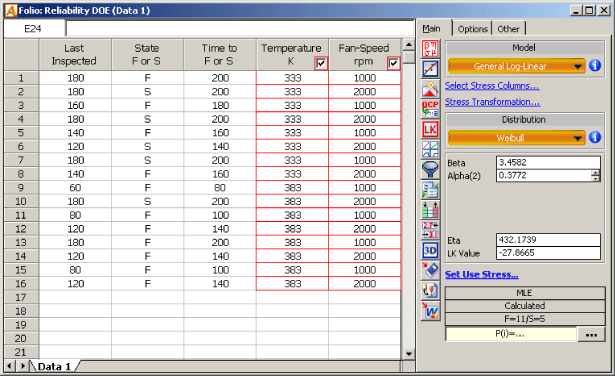
ALTA allows for modeling of the nature of relationship between life and stress. It is assumed that the relation between life of the product and temperature follows the Arrhenius relation while the relation between life and fan-speed follows the inverse power law relation [Accelerated Life Testing Reference]. Using these relations ALTA fits the following model for the data in the figure below:
- [math]\displaystyle{ \eta =\exp [-0.4322+1037.2886\frac{1}{\text{Temp}}+0.3772\cdot \ln (\text{Fan-Speed})]\,\! }[/math]
Based on this model the B10 life of the product at the use conditions is obtained as shown next. The Weibull reliability equation is:
- [math]\displaystyle{ R(t)=\exp \left[ -{{(\frac{t}{\eta })}^{Beta}} \right]\,\! }[/math]
Substituting the value of [math]\displaystyle{ \eta \,\! }[/math] from the fitted model and the value of [math]\displaystyle{ Beta(=3.4582)\,\! }[/math] as obtained from ALTA, the reliability equation becomes:
- [math]\displaystyle{ R(t)=\exp -{{\left[ \frac{t}{\exp [-0.4322+1037.2886\tfrac{1}{\text{Temp}}+0.3772\cdot \ln (\text{Fan-Speed})]} \right]}^{3.4582}}\,\! }[/math]
Finally, substituting the use conditions (Temp [math]\displaystyle{ =298\,\! }[/math] [math]\displaystyle{ K\,\! }[/math], Fan-Speed [math]\displaystyle{ =3000\,\! }[/math] [math]\displaystyle{ rpm\,\! }[/math]) and the desired reliability value of 90%, the B10 life is obtained:
- [math]\displaystyle{ \begin{align} 0.90= & \exp -{{\left[ \frac{t}{\exp [-0.4322+1037.2886\tfrac{1}{298}+0.3772\cdot \ln (3000)]} \right]}^{3.4582}} \\ t= & 225.4482 \end{align}\,\! }[/math]
Therefore, at the use conditions, the B10 life of the product is 225 time units. This result and other reliability metrics can be directly obtained from ALTA.
Single Factor R-DOE Analysis
DOE++ also allows for the analysis of single factor R-DOE experiments. This analysis is similar to the analysis of single factor designed experiments mentioned in Two Level Factorial Experiments. In single factor R-DOE analysis, the focus is on discovering whether change in the level of a factor affects reliability and how each of the factor levels are different from the other levels. The analysis models and calculations are similar to multi-factor R-DOE analysis.
Example
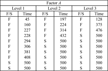
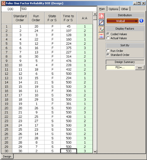
To illustrate single factor R-DOE analysis, consider the data in the table where life data readings for a product are taken at three levels of a certain factor, [math]\displaystyle{ A\,\! }[/math]. (Factor [math]\displaystyle{ A\,\! }[/math] may be thought of as a stress that is thought to affect life, three different designs of the same product, the same product manufactured by three different machines or operators, etc.) The goal of the experiment is to see if there is a change in life due to a change in the levels of the factor. The data from this experiment are shown in the figure below.
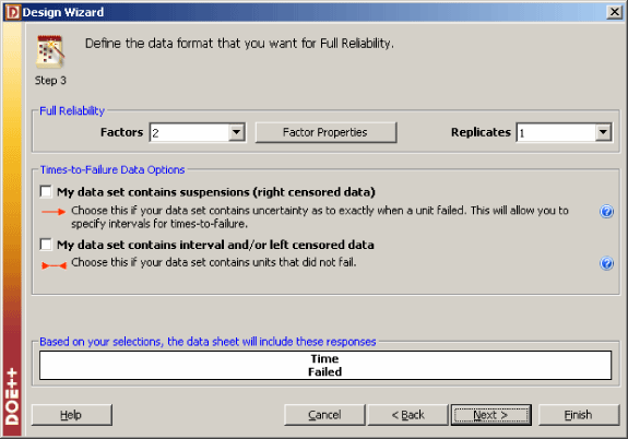
The data is entered into a folio that is configured for R-DOE analysis, as shown next.
The life of the product is assumed to follow the Weibull distribution. Therefore, the life characteristic to be used in the R-DOE analysis is the scale parameter, [math]\displaystyle{ \eta \,\! }[/math]. Since factor [math]\displaystyle{ A\,\! }[/math] has three levels, the model for the life characteristic, [math]\displaystyle{ \eta \,\! }[/math], is:
- [math]\displaystyle{ \ln ({{\eta }_{i}})={{\beta }_{0}}+{{\beta }_{1}}{{x}_{i1}}+{{\beta }_{2}}{{x}_{i2}}\,\! }[/math]
where [math]\displaystyle{ {{\beta }_{0}}\,\! }[/math] is the intercept, [math]\displaystyle{ {{\beta }_{1}}\,\! }[/math] is the effect coefficient for the first level of the factor ([math]\displaystyle{ {{\beta }_{1}}\,\! }[/math] is represented as "A[1]" in DOE++) and [math]\displaystyle{ {{\beta }_{2}}\,\! }[/math] is the effect coefficient for the second level of the factor ([math]\displaystyle{ {{\beta }_{2}}\,\! }[/math] is represented as "A[2]" in DOE++). Two indicator variables, [math]\displaystyle{ {{x}_{1}}\,\! }[/math] and [math]\displaystyle{ {{x}_{2}},\,\! }[/math] are the used to represent the three levels of factor [math]\displaystyle{ A\,\! }[/math] such that:
- [math]\displaystyle{ \begin{align} & {{x}_{1}}= & 1,\text{ }{{x}_{2}}=0\text{ Level 1 Effect} \\ & {{x}_{1}}= & 0,\text{ }{{x}_{2}}=1\text{ Level 2 Effect} \\ & {{x}_{1}}= & -1,\text{ }{{x}_{2}}=-1\text{ Level 3 Effect} \end{align}\,\! }[/math]
The following hypothesis test needs to be carried out in this example:
- [math]\displaystyle{ \begin{align} & {{H}_{0}}: & {{\theta }_{i}}=0 \\ & {{H}_{1}}: & {{\theta }_{i}}\ne 0 \end{align}\,\! }[/math]
where [math]\displaystyle{ {{\theta }_{i}}=[{{\beta }_{1}},{{\beta }_{2}}{]}'\,\! }[/math]. The statistic for this test is:
- [math]\displaystyle{ LR=-2\ln \frac{L({{{\hat{\theta }}}_{(-i)}})}{L(\hat{\theta })}\,\! }[/math]
where [math]\displaystyle{ L(\hat{\theta })\,\! }[/math] is the value of the likelihood function corresponding to the full model, and [math]\displaystyle{ L({{\hat{\theta }}_{(-i)}})\,\! }[/math] is the likelihood value for the reduced model. To calculate the statistic for this test, the MLE estimates of the parameters must be obtained.
MLE Estimates
Following the procedure used in the analysis of multi-factor R-DOE experiments, MLE estimates of the parameters are obtained by differentiating the log-likelihood function [math]\displaystyle{ \Lambda \,\! }[/math]:
- [math]\displaystyle{ \begin{align} & \Lambda = & \underset{i\epsilon 1}{\overset{{{F}_{e}}}{\mathop{\sum }}}\,\ln \left[ \frac{Beta}{{{\eta }_{i}}}{{\left( \frac{{{t}_{i}}}{{{\eta }_{i}}} \right)}^{Beta-1}}\exp \left[ -{{\left( \frac{{{t}_{i}}}{{{\eta }_{i}}} \right)}^{Beta}} \right] \right] \\ & & +\underset{i\epsilon 1}{\overset{{{S}_{e}}}{\mathop{\sum }}}\,\left[ -{{\left( \frac{{{t}_{i}}}{{{\eta }_{i}}} \right)}^{Beta}} \right] \\ & & +\underset{i\epsilon 1}{\overset{FI}{\mathop{\sum }}}\,\ln \left[ \exp \left[ -{{\left( \frac{t_{i}^{2}}{{{\eta }_{i}}} \right)}^{Beta}} \right]-\exp \left[ -{{\left( \frac{t_{i}^{1}}{{{\eta }_{i}}} \right)}^{Beta}} \right] \right] \end{align}\,\! }[/math]
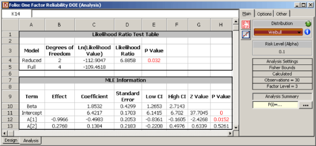
Substituting [math]\displaystyle{ {{\eta }_{i}}\,\! }[/math] from the model for the life characteristic [math]\displaystyle{ \eta\,\! }[/math] and setting the partial derivatives [math]\displaystyle{ \partial \Lambda /\partial {{\theta }_{i}}\,\! }[/math] to zero, the parameter estimates are obtained as [math]\displaystyle{ \hat{B}eta=1.8532\,\! }[/math], [math]\displaystyle{ {{\hat{\beta }}_{0}}=6.4217\,\! }[/math], [math]\displaystyle{ {{\hat{\beta }}_{1}}=-0.4983\,\! }[/math] and [math]\displaystyle{ {{\hat{\beta }}_{2}}=0.1384\,\! }[/math]. These parameters are shown in the figure below in the MLE Information table.
Likelihood Ratio Test
Knowing the MLE estimates, the likelihood ratio test for the significance of factor [math]\displaystyle{ A\,\! }[/math] can be carried out. The likelihood value for the full model, [math]\displaystyle{ L(\hat{\theta })\,\! }[/math], is the value of the likelihood function corresponding to the model [math]\displaystyle{ \ln ({{\eta }_{i}})={{\beta }_{0}}+{{\beta }_{1}}{{x}_{i1}}+{{\beta }_{2}}{{x}_{i2}}\,\! }[/math]:
- [math]\displaystyle{ \begin{align} L(\hat{\theta })= & L(\hat{B}eta,{{{\hat{\beta }}}_{0}},{{{\hat{\beta }}}_{1}},{{{\hat{\beta }}}_{2}}) \\ = & 9.2E-50 \end{align}\,\! }[/math]
The likelihood value for the reduced model, [math]\displaystyle{ L({{\hat{\theta }}_{(-i)}})\,\! }[/math], is the value of the likelihood function corresponding to the model [math]\displaystyle{ \ln ({{\eta }_{i}})={{\beta }_{0}}\,\! }[/math]:
- [math]\displaystyle{ \begin{align} L({{{\hat{\theta }}}_{(-i)}})= & L(\hat{B}eta,{{{\hat{\beta }}}_{0}}) \\ = & 2.9E-48 \end{align}\,\! }[/math]
Then the likelihood ratio is:
- [math]\displaystyle{ \begin{align} LR= & -2\ln \frac{L({{{\hat{\theta }}}_{(-i)}})}{L(\hat{\theta })} \\ = & 6.8858 \end{align}\,\! }[/math]
If the null hypothesis, [math]\displaystyle{ {{H}_{0}}\,\! }[/math], is true then the likelihood ratio will follow the chi-squared distribution. The number of degrees of freedom for this distribution is equal to the difference in the number of parameters between the full and the reduced model. In this case, this difference is 2. The [math]\displaystyle{ p\,\! }[/math] value corresponding to the likelihood ratio on the chi-squared distribution with two degrees of freedom is:
- [math]\displaystyle{ \begin{align} p\text{ }value= & 1-P(\chi _{2}^{2}\lt LR) \\ = & 1-0.968 \\ = & 0.032 \end{align}\,\! }[/math]
Assuming that the desired significance is 0.1, since [math]\displaystyle{ p\,\! }[/math] [math]\displaystyle{ value\lt 0.1\,\! }[/math], [math]\displaystyle{ {{H}_{0}}:{{\theta }_{i}}=0\,\! }[/math] is rejected it is concluded that, at a significance of 0.1, at least one of the parameters, [math]\displaystyle{ {{\beta }_{1}}\,\! }[/math] or [math]\displaystyle{ {{\beta }_{2}}\,\! }[/math], is non-zero. Therefore, factor [math]\displaystyle{ A\,\! }[/math] affects the life of the product. This result is shown in the Likelihood Ratio Test table in the figure above.
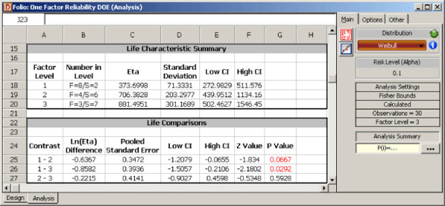
Additional results for single factor R-DOE analysis obtained from DOE ++ include information on the life characteristic and comparison of life characteristics at different levels of the factor.
Life Characteristic Summary Results
Results in the Life Characteristic Summary table include information about the life characteristic corresponding to each treatment level of the factor. If [math]\displaystyle{ \ln ({{\eta }_{i}})\,\! }[/math] is represented as [math]\displaystyle{ E({{y}_{i}})\,\! }[/math], then the model for the life characteristic [math]\displaystyle{ \eta\,\! }[/math] can be written as:
- [math]\displaystyle{ E({{y}_{i}})={{\beta }_{0}}+{{\beta }_{1}}{{x}_{i1}}+{{\beta }_{2}}{{x}_{i2}}\,\! }[/math]
The respective equations for all three treatment levels for a single replicate of the experiment can be expressed in matrix notation as:
- [math]\displaystyle{ E(y)=X\beta \,\! }[/math]
where:
- [math]\displaystyle{ E(y)=\left[ \begin{matrix} E({{y}_{1}}) \\ E({{y}_{2}}) \\ E({{y}_{3}}) \\ \end{matrix} \right]\text{ }X=\left[ \begin{matrix} 1 & 1 & 0 \\ 1 & 0 & 1 \\ 1 & -1 & -1 \\ \end{matrix} \right]\text{ }\beta =\left[ \begin{matrix} {{\beta }_{0}} \\ {{\beta }_{1}} \\ {{\beta }_{2}} \\ \end{matrix} \right]\,\! }[/math]
Knowing [math]\displaystyle{ {{\hat{\beta }}_{0}}\,\! }[/math], [math]\displaystyle{ {{\hat{\beta }}_{1}}\,\! }[/math] and [math]\displaystyle{ {{\hat{\beta }}_{2}}\,\! }[/math], the predicted value of the life characteristic at any level can be obtained. For example, for the second level:
- [math]\displaystyle{ \begin{align} E({{{\hat{y}}}_{2}})= & {{{\hat{\beta }}}_{0}}+{{{\hat{\beta }}}_{2}} \\ or\text{ }\ln ({{{\hat{\eta }}}_{2}})= & {{{\hat{\beta }}}_{0}}+{{{\hat{\beta }}}_{2}} \\ = & 6.421743+0.138414 \\ = & 6.560157 \end{align}\,\! }[/math]
Thus:
- [math]\displaystyle{ \begin{align} {{{\hat{\eta }}}_{2}}= & \exp (6.560157) \\ = & 706.3828 \end{align}\,\! }[/math]
The variance for the predicted values of life characteristic can be calculated using the following equation:
- [math]\displaystyle{ Var(y)=XVar(\hat{\beta }){{X}^{\prime }}\,\! }[/math]
where [math]\displaystyle{ Var(\hat{\beta })\,\! }[/math] is the variance-covariance matrix for [math]\displaystyle{ {{\hat{\beta }}_{0}}\,\! }[/math], [math]\displaystyle{ {{\hat{\beta }}_{1}}\,\! }[/math] and [math]\displaystyle{ {{\hat{\beta }}_{2}}\,\! }[/math]. Substituting the required values:
From the previous matrix, [math]\displaystyle{ Var({{\hat{y}}_{2}})=0.0829\,\! }[/math]. Therefore, the 90% confidence interval ([math]\displaystyle{ \alpha =0.1\,\! }[/math]) on [math]\displaystyle{ {{\hat{y}}_{2}}\,\! }[/math] is:
- [math]\displaystyle{ \begin{align} CI\text{ }on\text{ }{{{\hat{y}}}_{2}}= & E({{{\hat{y}}}_{2}})\pm {{z}_{\alpha /2}}\sqrt{Var({{{\hat{y}}}_{2}})} \\ = & E({{{\hat{y}}}_{2}})\pm {{z}_{0.05}}\sqrt{Var({{{\hat{y}}}_{2}})} \\ = & 6.560157\pm 1.645\sqrt{0.0829} \\ = & 6.0867\text{ }and\text{ }7.0336 \end{align}\,\! }[/math]
Since [math]\displaystyle{ {{\hat{y}}_{2}}=\ln ({{\hat{\eta }}_{2}}),\,\! }[/math] the 90% confidence interval on [math]\displaystyle{ {{\hat{\eta }}_{2}}\,\! }[/math] is:
- [math]\displaystyle{ \begin{align} CI\text{ }on\text{ }{{{\hat{\eta }}}_{2}}= & \exp (6.0867)\text{ }and\text{ }\exp (7.0336) \\ = & 439.9\text{ }and\text{ }1134.1 \end{align}\,\! }[/math]
Results for other levels can be calculated in a similar manner and are shown in the figure below.
Life Comparisons Results
Results under Life Comparisons include information on how life is different at a level in comparison to any other level of the factor. For example, the difference between the predicted values of life at levels 1 and 2 is (in terms of the logarithmic transformation):
- [math]\displaystyle{ \begin{align} E({{{\hat{y}}}_{1}})-E({{{\hat{y}}}_{2}})= & 5.923453-6.560157 \\ = & -0.6367 \end{align}\,\! }[/math]
The pooled standard error for this difference can be obtained as:
- [math]\displaystyle{ \begin{align} Pooled\text{ }Std.\text{ }Error= & \sqrt{Var({{{\hat{y}}}_{1}}-{{{\hat{y}}}_{2}})} \\ = & \sqrt{Var({{{\hat{y}}}_{1}})+Var({{{\hat{y}}}_{2}})} \\ = & \sqrt{0.0366+0.0831} \\ = & 0.3454 \end{align}\,\! }[/math]
If the covariance between [math]\displaystyle{ {{\hat{y}}_{1}}\,\! }[/math] and [math]\displaystyle{ {{\hat{y}}_{2}}\,\! }[/math] is taken into account, then the pooled standard error is:
- [math]\displaystyle{ \begin{align} Pooled\text{ }Std.\text{ }Error= & \sqrt{Var({{{\hat{y}}}_{1}}-{{{\hat{y}}}_{2}})} \\ = & \sqrt{Var({{{\hat{y}}}_{1}})+Var({{{\hat{y}}}_{2}})-2\cdot Cov({{{\hat{y}}}_{1}},{{{\hat{y}}}_{2}})} \\ = & \sqrt{0.0364+0.0829-2\cdot (-0.0006)} \\ = & 0.3471 \end{align}\,\! }[/math]
This is the value displayed by DOE++. Knowing the pooled standard error, the confidence interval on the difference can be calculated. The 90% confidence interval on the difference in (logarithmic) life between levels 1 and 2 of factor [math]\displaystyle{ A\,\! }[/math] is:
- [math]\displaystyle{ \begin{align} = & \{E({{{\hat{y}}}_{1}})-E({{{\hat{y}}}_{2}})\}\pm {{z}_{\alpha /2}}\cdot Pooled\text{ }Std.\text{ }Error \\ = & \{E({{{\hat{y}}}_{1}})-E({{{\hat{y}}}_{2}})\}\pm {{z}_{0.05}}\cdot Pooled\text{ }Std.\text{ }Error \\ = & -0.6367\pm 1.645\cdot 0.3471 \\ = & \text{ }-1.208\text{ }and\text{ }-0.066 \end{align}\,\! }[/math]
Since the confidence interval does not include zero it can be concluded that the two levels are significantly different at [math]\displaystyle{ \alpha =0.1\,\! }[/math]. Another way to test for the significance of the difference in levels is to observe the [math]\displaystyle{ p\,\! }[/math] value. The [math]\displaystyle{ z\,\! }[/math] statistic corresponding to this difference is:
- [math]\displaystyle{ \begin{align} {{z}_{(1-2)}}= & \frac{E({{{\hat{y}}}_{1}})-E({{{\hat{y}}}_{2}})}{Pooled\text{ }Std.\text{ }Error} \\ = & \frac{-0.6367}{0.3471} \\ = & -1.834 \end{align}\,\! }[/math]
The [math]\displaystyle{ p\,\! }[/math] value corresponding to this statistic, based on the standard normal distribution, is:
- [math]\displaystyle{ \begin{align} p\text{ }value= & 2\cdot (1-P(Z\lt |-1.8335|) \\ = & 2\cdot (0.03336) \\ = & 0.0667 \end{align}\,\! }[/math]
Since [math]\displaystyle{ p\,\! }[/math] [math]\displaystyle{ value\lt \alpha ,\,\! }[/math] it can be concluded that the levels are significantly different at [math]\displaystyle{ \alpha =0.1\,\! }[/math]. The results for other levels can be calculated in a similar manner and are shown in the figure above.

