Example Using a Distribution to Approximate the CDF: Difference between revisions
Kate Racaza (talk | contribs) No edit summary |
No edit summary |
||
| Line 9: | Line 9: | ||
Components | Components <math>A\,\!</math> through <math>E\,\!</math> are Weibull distributed with <math>\beta =1.2\,\!</math> and <math>\eta =1230\,\!</math> hours. The starting and ending blocks cannot fail. Compute a single Weibull distribution approximation for the system.</noinclude><includeonly>Compute a single Weibull distribution approximation for the parallel system in the previous example.</includeonly> | ||
<!-- THIS EXAMPLE USES THE DATA SET FROM ANOTHER EXAMPLE. IF YOU EDIT THE DATA SET ON THIS PAGE, YOU MUST ALSO EDIT THE DATA SET IN THE PAGE: Time-Dependent System Reliability for Components in Parallel --> | <!-- THIS EXAMPLE USES THE DATA SET FROM ANOTHER EXAMPLE. IF YOU EDIT THE DATA SET ON THIS PAGE, YOU MUST ALSO EDIT THE DATA SET IN THE PAGE: Time-Dependent System Reliability for Components in Parallel --> | ||
'''Solution''' | '''Solution''' | ||
Assume that the system can be approximated by a 2-parameter Weibull distribution with | Assume that the system can be approximated by a 2-parameter Weibull distribution with <math>\beta =2.02109\,\!</math> and <math>\eta =1123.51\,\!</math>. In BlockSim, this is accomplished by representing the entire system as one distribution. To do this, click the '''Distribution fit''' area on the diagram's control panel, as shown next. | ||
| Line 24: | Line 24: | ||
[[Image:Fig 5.12.PNG|center|450px|<div align="center"> Distribution Estimator.</div>]] | [[Image:Fig 5.12.PNG|center|450px|<div align="center"> Distribution Estimator.</div>]] | ||
When you analyze the diagram, BlockSim will generate a number of system failure times based on the system's reliability function. The system's reliability function can be used to solve for a time value associated with an unreliability value. For example, consider an unreliability value of | When you analyze the diagram, BlockSim will generate a number of system failure times based on the system's reliability function. The system's reliability function can be used to solve for a time value associated with an unreliability value. For example, consider an unreliability value of <math>F(t)=0.11\,\!</math>. Using the system's reliability equation, the corresponding time-to-failure for a 0.11 unreliability is 389.786 hours. The distribution of the generated time values can then be fitted to a probability distribution function. | ||
When enough points have been generated, the selected distribution will be fitted to the generated data set and the distribution's parameters will be calculated. In addition, if ReliaSoft's Weibull++ is installed, the fit of the distribution can be analyzed using a Weibull++ standard folio, as shown in the next figure. It is recommended that the analyst examine the fit to ascertain the applicability of the approximation. | When enough points have been generated, the selected distribution will be fitted to the generated data set and the distribution's parameters will be calculated. In addition, if ReliaSoft's Weibull++ is installed, the fit of the distribution can be analyzed using a Weibull++ standard folio, as shown in the next figure. It is recommended that the analyst examine the fit to ascertain the applicability of the approximation. | ||
Revision as of 21:19, 17 September 2012
New format available! This reference is now available in a new format that offers faster page load, improved display for calculations and images and more targeted search.
As of January 2024, this Reliawiki page will not continue to be updated. Please update all links and bookmarks to the latest references at BlockSim examples and BlockSim reference examples.
This example appears in the System Analysis Reference book.
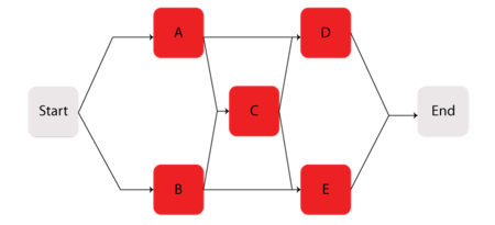
Consider the system shown next.
Components [math]\displaystyle{ A\,\! }[/math] through [math]\displaystyle{ E\,\! }[/math] are Weibull distributed with [math]\displaystyle{ \beta =1.2\,\! }[/math] and [math]\displaystyle{ \eta =1230\,\! }[/math] hours. The starting and ending blocks cannot fail. Compute a single Weibull distribution approximation for the system.
Solution
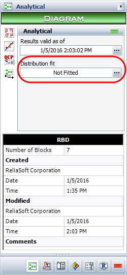
Assume that the system can be approximated by a 2-parameter Weibull distribution with [math]\displaystyle{ \beta =2.02109\,\! }[/math] and [math]\displaystyle{ \eta =1123.51\,\! }[/math]. In BlockSim, this is accomplished by representing the entire system as one distribution. To do this, click the Distribution fit area on the diagram's control panel, as shown next.
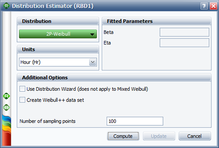
This opens the Distribution Estimator window, which allows you to select a distribution to represent the data.
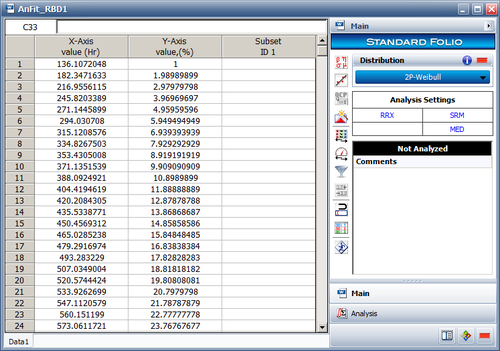
When you analyze the diagram, BlockSim will generate a number of system failure times based on the system's reliability function. The system's reliability function can be used to solve for a time value associated with an unreliability value. For example, consider an unreliability value of [math]\displaystyle{ F(t)=0.11\,\! }[/math]. Using the system's reliability equation, the corresponding time-to-failure for a 0.11 unreliability is 389.786 hours. The distribution of the generated time values can then be fitted to a probability distribution function.
When enough points have been generated, the selected distribution will be fitted to the generated data set and the distribution's parameters will be calculated. In addition, if ReliaSoft's Weibull++ is installed, the fit of the distribution can be analyzed using a Weibull++ standard folio, as shown in the next figure. It is recommended that the analyst examine the fit to ascertain the applicability of the approximation.


