The Gamma Distribution

The gamma distribution is a flexible life distribution model that may offer a good fit to some sets of failure data. It is not, however, widely used as a life distribution model for common failure mechanisms. The gamma distribution does arise naturally as the time-to-first-fail distribution for a system with standby exponentially distributed backups, and is also a good fit for the sum of independent exponential random variables. The gamma distribution is sometimes called the Erlang distribution, which is used frequently in queuing theory applications [32].

The Gamma Probability Density Function

The [math]\displaystyle{ pdf }[/math] of the gamma distribution is given by:

[math]\displaystyle{ f(t)=\frac{{{e}^{kz-{{e}^{z}}}}}{t\Gamma (k)} }[/math]

where:

[math]\displaystyle{ \begin{align} z=\ln (t)-\mu \end{align} }[/math]

and:

[math]\displaystyle{ \begin{align} & {{e}^{\mu }}= \text{scale parameter} \\ & k= \text{shape parameter} \end{align} }[/math]

where [math]\displaystyle{ 0\lt t\lt \infty }[/math] , [math]\displaystyle{ -\infty \lt \mu \lt \infty }[/math] and [math]\displaystyle{ k\gt 0 }[/math] .

The Gamma Reliability Function

The reliability for a mission of time [math]\displaystyle{ t\,\! }[/math] for the gamma distribution is:

[math]\displaystyle{ \begin{align} R=1-{{\Gamma }_{I}}(k;{{e}^{z}}) \end{align} }[/math]

The Gamma Mean, Median and Mode

The gamma mean or MTTF is:

[math]\displaystyle{ \overline{T}=k{{e}^{\mu }} }[/math]

The mode exists if [math]\displaystyle{ k\gt 1\,\! }[/math] and is given by:

[math]\displaystyle{ \tilde{T}=(k-1){{e}^{\mu }} }[/math]

The median is:

[math]\displaystyle{ \widehat{T}={{e}^{\mu +\ln (\Gamma _{I}^{-1}(0.5;k))}} }[/math]

The Gamma Standard Deviation

The standard deviation for the gamma distribution is:

[math]\displaystyle{ {{\sigma }_{T}}=\sqrt{k}{{e}^{\mu }} }[/math]

The Gamma Reliable Life

The gamma reliable life is:

[math]\displaystyle{ {{T}_{R}}={{e}^{\mu +\ln (\Gamma _{1}^{-1}(1-R;k))}} }[/math]

The Gamma Failure Rate Function

The instantaneous gamma failure rate is given by:

[math]\displaystyle{ \lambda =\frac{{{e}^{kz-{{e}^{z}}}}}{t\Gamma (k)(1-{{\Gamma }_{I}}(k;{{e}^{z}}))} }[/math]

Characteristics of the Gamma Distribution

Some of the specific characteristics of the gamma distribution are the following:

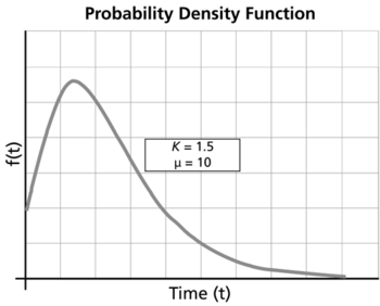
For [math]\displaystyle{ k\gt 1 }[/math] :

• As [math]\displaystyle{ t\to 0,\infty }[/math] , [math]\displaystyle{ f(t)\to 0. }[/math]

• [math]\displaystyle{ f(t) }[/math] increases from 0 to the mode value and decreases thereafter.

• If [math]\displaystyle{ k\le 2 }[/math] then [math]\displaystyle{ pdf }[/math] has one inflection point at [math]\displaystyle{ t={{e}^{\mu }}\sqrt{k-1}( }[/math] [math]\displaystyle{ \sqrt{k-1}+1). }[/math]

• If [math]\displaystyle{ k\gt 2 }[/math] then [math]\displaystyle{ pdf }[/math] has two inflection points for [math]\displaystyle{ t={{e}^{\mu }}\sqrt{k-1}( }[/math] [math]\displaystyle{ \sqrt{k-1}\pm 1). }[/math]

• For a fixed [math]\displaystyle{ k }[/math] , as [math]\displaystyle{ \mu }[/math] increases, the [math]\displaystyle{ pdf }[/math] starts to look more like a straight angle.

• As [math]\displaystyle{ t\to \infty ,\lambda (t)\to \tfrac{1}{{{e}^{\mu }}}. }[/math]

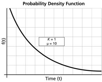
For [math]\displaystyle{ k=1 }[/math] :

• Gamma becomes the exponential distribution.

• As [math]\displaystyle{ t\to 0 }[/math] , [math]\displaystyle{ f(T)\to \tfrac{1}{{{e}^{\mu }}}. }[/math]

• As [math]\displaystyle{ t\to \infty ,f(t)\to 0. }[/math]

• The [math]\displaystyle{ pdf }[/math] decreases monotonically and is convex.

• [math]\displaystyle{ \lambda (t)\equiv \tfrac{1}{{{e}^{\mu }}} }[/math] . [math]\displaystyle{ \lambda (t) }[/math] is constant.

• The mode does not exist.

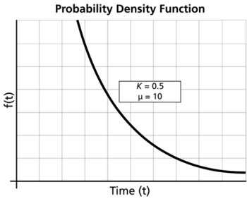
For [math]\displaystyle{ 0\lt k\lt 1 }[/math] :

• As [math]\displaystyle{ t\to 0 }[/math] , [math]\displaystyle{ f(t)\to \infty . }[/math]

• As [math]\displaystyle{ t\to \infty ,f(t)\to 0. }[/math]

• As [math]\displaystyle{ t\to \infty ,\lambda (t)\to \tfrac{1}{{{e}^{\mu }}}. }[/math]

• The [math]\displaystyle{ pdf }[/math] decreases monotonically and is convex.

• As [math]\displaystyle{ \mu }[/math] increases, the [math]\displaystyle{ pdf }[/math] gets stretched out to the right and its height decreases, while maintaining its shape.

• As [math]\displaystyle{ \mu }[/math] decreases, the [math]\displaystyle{ pdf }[/math] shifts towards the left and its height increases.

• The mode does not exist.

Confidence Bounds

The only method available in Weibull++ for confidence bounds for the gamma distribution is the Fisher matrix, which is described next. The complete derivations were presented in detail (for a general function) in the Confidence Bounds chapter.

Bounds on the Parameters

The lower and upper bounds on the mean, [math]\displaystyle{ \widehat{\mu } }[/math] , are estimated from:

[math]\displaystyle{ \begin{align} & {{\mu }_{U}}= & \widehat{\mu }+{{K}_{\alpha }}\sqrt{Var(\widehat{\mu })}\text{ (upper bound)} \\ & {{\mu }_{L}}= & \widehat{\mu }-{{K}_{\alpha }}\sqrt{Var(\widehat{\mu })}\text{ (lower bound)} \end{align} }[/math]

Since the standard deviation, [math]\displaystyle{ \widehat{\sigma } }[/math] , must be positive, [math]\displaystyle{ \ln (\widehat{\sigma }) }[/math] is treated as normally distributed and the bounds are estimated from:

[math]\displaystyle{ \begin{align} & {{k}_{U}}= & \widehat{k}\cdot {{e}^{\tfrac{{{K}_{\alpha }}\sqrt{Var(\widehat{k})}}{{\hat{k}}}}}\text{ (upper bound)} \\ & {{k}_{L}}= & \frac{\widehat{\sigma }}{{{e}^{\tfrac{{{K}_{\alpha }}\sqrt{Var(\widehat{k})}}{\widehat{k}}}}}\text{ (lower bound)} \end{align} }[/math]

where [math]\displaystyle{ {{K}_{\alpha }} }[/math] is defined by:

[math]\displaystyle{ \alpha =\frac{1}{\sqrt{2\pi }}\int_{{{K}_{\alpha }}}^{\infty }{{e}^{-\tfrac{{{t}^{2}}}{2}}}dt=1-\Phi ({{K}_{\alpha }}) }[/math]

If [math]\displaystyle{ \delta }[/math] is the confidence level, then [math]\displaystyle{ \alpha =\tfrac{1-\delta }{2} }[/math] for the two-sided bounds and [math]\displaystyle{ \alpha =1-\delta }[/math] for the one-sided bounds.

The variances and covariances of [math]\displaystyle{ \widehat{\mu } }[/math] and [math]\displaystyle{ \widehat{k} }[/math] are estimated from the Fisher matrix, as follows:

[math]\displaystyle{ \left( \begin{matrix} \widehat{Var}\left( \widehat{\mu } \right) & \widehat{Cov}\left( \widehat{\mu },\widehat{k} \right) \\ \widehat{Cov}\left( \widehat{\mu },\widehat{k} \right) & \widehat{Var}\left( \widehat{k} \right) \\ \end{matrix} \right)=\left( \begin{matrix} -\tfrac{{{\partial }^{2}}\Lambda }{\partial {{\mu }^{2}}} & -\tfrac{{{\partial }^{2}}\Lambda }{\partial \mu \partial k} \\ {} & {} \\ -\tfrac{{{\partial }^{2}}\Lambda }{\partial \mu \partial k} & -\tfrac{{{\partial }^{2}}\Lambda }{\partial {{k}^{2}}} \\ \end{matrix} \right)_{\mu =\widehat{\mu },k=\widehat{k}}^{-1} }[/math]

[math]\displaystyle{ \Lambda }[/math] is the log-likelihood function of the gamma distribution, described in Parameter Estimation and Appendix D

Bounds on Reliability

The reliability of the gamma distribution is:

[math]\displaystyle{ \widehat{R}(t;\hat{\mu },\hat{k})=1-{{\Gamma }_{I}}(\widehat{k};{{e}^{\widehat{z}}}) }[/math]

where:

[math]\displaystyle{ \widehat{z}=\ln (t)-\widehat{\mu } }[/math]

The upper and lower bounds on reliability are:

[math]\displaystyle{ {{R}_{U}}=\frac{\widehat{R}}{\widehat{R}+(1-\widehat{R})\exp (\tfrac{-{{K}_{\alpha }}\sqrt{Var(\widehat{R})\text{ }}}{\widehat{R}(1-\widehat{R})})}\text{ (upper bound)} }[/math]

[math]\displaystyle{ {{R}_{L}}=\frac{\widehat{R}}{\widehat{R}+(1-\widehat{R})\exp (\tfrac{{{K}_{\alpha }}\sqrt{Var(\widehat{R})\text{ }}}{\widehat{R}(1-\widehat{R})})}\text{ (lower bound)} }[/math]

where:

[math]\displaystyle{ Var(\widehat{R})={{(\frac{\partial R}{\partial \mu })}^{2}}Var(\widehat{\mu })+2(\frac{\partial R}{\partial \mu })(\frac{\partial R}{\partial k})Cov(\widehat{\mu },\widehat{k})+{{(\frac{\partial z}{\partial k})}^{2}}Var(\widehat{k}) }[/math]

Bounds on Time

The bounds around time for a given gamma percentile (unreliability) are estimated by first solving the reliability equation with respect to time, as follows:

[math]\displaystyle{ \widehat{T}(\widehat{\mu },\widehat{\sigma })=\widehat{\mu }+\widehat{\sigma }z }[/math]

where:

[math]\displaystyle{ z=\ln (-\ln (R)) }[/math]

[math]\displaystyle{ Var(\widehat{T})={{(\frac{\partial T}{\partial \mu })}^{2}}Var(\widehat{\mu })+2(\frac{\partial T}{\partial \mu })(\frac{\partial T}{\partial \sigma })Cov(\widehat{\mu },\widehat{\sigma })+{{(\frac{\partial T}{\partial \sigma })}^{2}}Var(\widehat{\sigma }) }[/math]

or:

[math]\displaystyle{ Var(\widehat{T})=Var(\widehat{\mu })+2\widehat{z}Cov(\widehat{\mu },\widehat{\sigma })+{{\widehat{z}}^{2}}Var(\widehat{\sigma }) }[/math]

The upper and lower bounds are then found by:

[math]\displaystyle{ \begin{align} & {{T}_{U}}= & \hat{T}+{{K}_{\alpha }}\sqrt{Var(\hat{T})}\text{ (Upper bound)} \\ & {{T}_{L}}= & \hat{T}-{{K}_{\alpha }}\sqrt{Var(\hat{T})}\text{ (Lower bound)} \end{align} }[/math]

General Example

24 units were reliability tested, and the following life test data were obtained:

61	50	67	49	53	62
53	61	43	65	53	56
62	56	58	55	58	48
66	44	48	58	43	40

Fitting the gamma distribution to this data, using maximum likelihood as the analysis method, gives the following parameters:

[math]\displaystyle{ \begin{align} & \hat{\mu }= 7.72E-02 \\ & \hat{k}= 50.4908 \end{align}\,\! }[/math]

Using rank regression on [math]\displaystyle{ X,\,\! }[/math] the estimated parameters are:

[math]\displaystyle{ \begin{align} & \hat{\mu }= 0.2915 \\ & \hat{k}= 41.1726 \end{align}\,\! }[/math]

Using rank regression on [math]\displaystyle{ Y,\,\! }[/math] the estimated parameters are:

[math]\displaystyle{ \begin{align} & \hat{\mu }= 0.2915 \\ & \hat{k}= 41.1726 \end{align}\,\! }[/math]