Bayesian-Weibull Lognormal Prior Example

New format available! This reference is now available in a new format that offers faster page load, improved display for calculations and images and more targeted search.

As of January 2024, this Reliawiki page will not continue to be updated. Please update all links and bookmarks to the latest references at Weibull examples and Weibull reference examples.

---

This example appears in the Life Data Analysis Reference book.

A manufacturer has tested prototypes of a modified product. The test was terminated at 2,000 hours, with only 2 failures observed from a sample size of 18. The following table shows the data.

Number of State	State of F or S	State End Time
1	F	1180
1	F	1842
16	S	2000

Because of the lack of failure data in the prototype testing, the manufacturer decided to use information gathered from prior tests on this product to increase the confidence in the results of the prototype testing. This decision was made because failure analysis indicated that the failure mode of the two failures is the same as the one that was observed in previous tests. In other words, it is expected that the shape of the distribution (beta) hasn't changed, but hopefully the scale (eta) has, indicating longer life. The 2-parameter Weibull distribution was used to model all prior tests results. The estimated beta (β) parameters of the prior test results are as follows:

Betas Obtained for Similar Mode
1.7
2.1
2.4
3.1
3.5

Solution

First, in order to fit the data to a Bayesian-Weibull model, a prior distribution for beta needs to be determined. Based on the beta values in the prior tests, the prior distribution for beta is found to be a lognormal distribution with μ = 0.9064, σ = 0.3325. (The values of the parameters can be obtained by entering the beta values into a Weibull++ standard folio and analyzing it using the lognormal distribution and the RRX analysis method.)

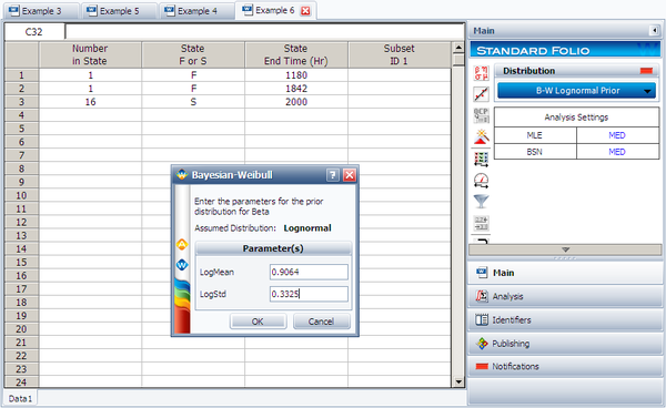
Next, enter the data from the prototype testing into a standard folio. On the control panel, choose the Bayesian-Weibull > B-W Lognormal Prior distribution. Click Calculate and enter the parameters of the lognormal distribution, as shown next.

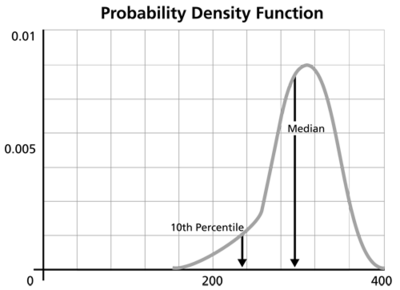
Click OK. The result is Beta (Median) = 2.361219 and Eta (Median) = 5321.631912 (by default Weibull++ returns the median values of the posterior distribution). Suppose that the reliability at 3,000 hours is the metric of interest in this example. Using the QCP, the reliability is calculated to be 76.97% at 3,000 hours. The following picture depicts the posterior [math]\displaystyle{ pdf }[/math] plot of the reliability at 3,000, with the corresponding median value as well as the 10th percentile value. The 10th percentile constitutes the 90% lower 1-sided bound on the reliability at 3,000 hours, which is calculated to be 50.77%.

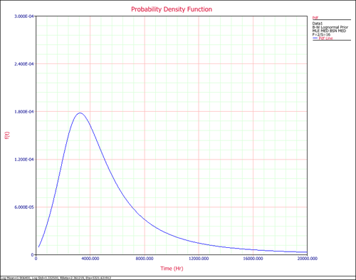
The [math]\displaystyle{ pdf }[/math] of the times-to-failure data can be plotted in Weibull++, as shown next: