Probability Plotting Example: Difference between revisions
No edit summary |
Lisa Hacker (talk | contribs) No edit summary |
||
| Line 1: | Line 1: | ||
<noinclude>{{Banner Weibull Examples}} | <noinclude>{{Banner Weibull Examples}} | ||
''This example appears in the [[ | ''This example appears in the [[The_Exponential_Distribution#Probability_Plotting|Life Data Analysis Reference book]]''. | ||
</noinclude> | </noinclude> | ||
Let's assume six identical units are reliability tested at the same application and operation | Let's assume six identical units are reliability tested at the same application and operation | ||
Revision as of 08:30, 6 August 2012
New format available! This reference is now available in a new format that offers faster page load, improved display for calculations and images and more targeted search.
As of January 2024, this Reliawiki page will not continue to be updated. Please update all links and bookmarks to the latest references at Weibull examples and Weibull reference examples.
This example appears in the Life Data Analysis Reference book.
Let's assume six identical units are reliability tested at the same application and operation stress levels. All of these units fail during the test after operating for the following times (in hours), [math]\displaystyle{ {{T}_{i}} }[/math] : 96, 257, 498, 763, 1051 and 1744.
The steps for determining the parameters of the exponential [math]\displaystyle{ pdf }[/math] representing the data, using probability plotting, are as follows:
Rank the times-to-failure in ascending order as shown next.
- [math]\displaystyle{ \begin{matrix} \text{Time-to-} & \text{Failure Order Number} \\ \text{failure, hr} & \text{out of a Sample Size of 6} \\ \text{96} & \text{1} \\ \text{257} & \text{2} \\ \text{498} & \text{3} \\ \text{763} & \text{4} \\ \text{1,051} & \text{5} \\ \text{1,744} & \text{6} \\ \end{matrix} }[/math]
Obtain their median rank plotting positions.
Median rank positions are used instead of other ranking methods because median ranks are at a specific confidence level (50%).
The times-to-failure, with their corresponding median ranks, are shown next:
- [math]\displaystyle{ \begin{matrix} \text{Time-to-} & \text{Median} \\ \text{failure, hr} & \text{Rank, }% \\ \text{96} & \text{10}\text{.91} \\ \text{257} & \text{26}\text{.44} \\ \text{498} & \text{42}\text{.14} \\ \text{763} & \text{57}\text{.86} \\ \text{1,051} & \text{73}\text{.56} \\ \text{1,744} & \text{89}\text{.10} \\ \end{matrix} }[/math]
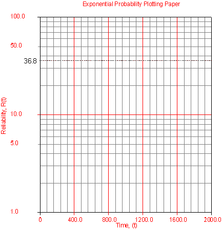
On an exponential probability paper, plot the times on the x-axis and their corresponding rank value on the y-axis. The next figure displays an example of an exponential probability paper. The paper is simply a log-linear paper.
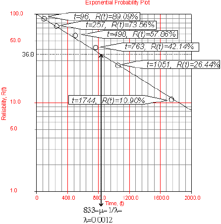
Draw the best possible straight line that goes through the [math]\displaystyle{ t=0 }[/math] and [math]\displaystyle{ (t)=100% }[/math] point and through the plotted points (as shown in the plot below).
At the [math]\displaystyle{ Q(t)=63.2% }[/math] or [math]\displaystyle{ R(t)=36.8% }[/math] ordinate point, draw a straight horizontal line until this line intersects the fitted straight line. Draw a vertical line through this intersection until it crosses the abscissa. The value at the intersection of the abscissa is the estimate of the mean. For this case, [math]\displaystyle{ \widehat{\mu }=833 }[/math] hr which means that [math]\displaystyle{ \lambda =\tfrac{1}{\mu }=0.0012 }[/math] (This is always at 63.2% because [math]\displaystyle{ (T)=1-{{e}^{-\tfrac{\mu }{\mu }}}=1-{{e}^{-1}}=0.632=63.2%). }[/math]
Now any reliability value for any mission time [math]\displaystyle{ t }[/math] can be obtained. For example, the reliability for a mission of 15 hr, or any other time, can now be obtained either from the plot or analytically.
To obtain the value from the plot, draw a vertical line from the abscissa, at [math]\displaystyle{ t=15 }[/math] hr, to the fitted line. Draw a horizontal line from this intersection to the ordinate and read [math]\displaystyle{ R(t) }[/math] . In this case, [math]\displaystyle{ R(t=15)=98.15% }[/math] . This can also be obtained analytically, from the exponential reliability function.


