Example Using Load Sharing Gates in Fault Trees: Difference between revisions
No edit summary |
No edit summary |
||
| Line 6: | Line 6: | ||
<br> | <br> | ||
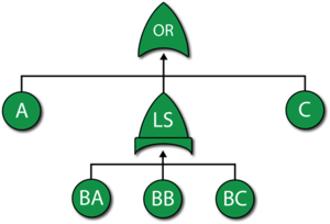
The first step is to create the fault tree as shown in figure below. Note that both an OR gate and a Load Sharing gate are used. | The first step is to create the fault tree as shown in the figure below. Note that both an OR gate and a Load Sharing gate are used. | ||
[[Image:10.7.png|center|300px| Fault tree for the example illustrating a Load Sharing gate.]] | [[Image:10.7.png|center|300px| Fault tree for the example illustrating a Load Sharing gate.]] | ||
Revision as of 08:43, 2 August 2012
New format available! This reference is now available in a new format that offers faster page load, improved display for calculations and images and more targeted search.
As of January 2024, this Reliawiki page will not continue to be updated. Please update all links and bookmarks to the latest references at BlockSim examples and BlockSim reference examples.
A component has five possible failure modes, [math]\displaystyle{ A }[/math] , [math]\displaystyle{ {{B}_{A}} }[/math] , [math]\displaystyle{ {{B}_{B}} }[/math] , [math]\displaystyle{ {{B}_{C}} }[/math] and [math]\displaystyle{ C }[/math] , and the [math]\displaystyle{ B }[/math] modes are interdependent. The system will fail if mode [math]\displaystyle{ A }[/math] occurs, mode [math]\displaystyle{ C }[/math] occurs or two out of the three [math]\displaystyle{ B }[/math] modes occur. Modes [math]\displaystyle{ A }[/math] and [math]\displaystyle{ C }[/math] have a Weibull distribution with [math]\displaystyle{ \beta =2 }[/math] and [math]\displaystyle{ \eta =10,000 }[/math] and [math]\displaystyle{ 15,000 }[/math] respectively. Events [math]\displaystyle{ {{B}_{A}} }[/math] , [math]\displaystyle{ {{B}_{B}} }[/math] and [math]\displaystyle{ {{B}_{C}} }[/math] have an exponential distribution with a mean of [math]\displaystyle{ 10,000 }[/math] hours. If any [math]\displaystyle{ B }[/math] event occurs (i.e., [math]\displaystyle{ {{B}_{A}} }[/math] , [math]\displaystyle{ {{B}_{B}} }[/math] or [math]\displaystyle{ {{B}_{C}} }[/math] ), the remaining [math]\displaystyle{ B }[/math] events are more likely to occur. Specifically, the mean times of the remaining [math]\displaystyle{ B }[/math] events are halved. Determine the reliability at [math]\displaystyle{ 1,000 }[/math] hours for this component.
Solution
The first step is to create the fault tree as shown in the figure below. Note that both an OR gate and a Load Sharing gate are used.
The next step is to define the properties for each event block and the Load Sharing gate. Setting the failure distributions for modes [math]\displaystyle{ A }[/math] and [math]\displaystyle{ C }[/math] is simple.
The more difficult part is setting the properties of the Load Sharing gate (which are the same as an RBD container) and the dependent load sharing events (which are the same as the contained blocks in an RBD). Based on the problem statement, the [math]\displaystyle{ B }[/math] modes are in a 2-out-of-3 load sharing redundancy. When all three are working (i.e., when no [math]\displaystyle{ B }[/math] mode has occurred), each block has an exponential distribution with [math]\displaystyle{ \mu =10,000 }[/math] . If one [math]\displaystyle{ B }[/math] mode occurs, then the two surviving units have an exponential distribution with [math]\displaystyle{ \mu =5,000. }[/math]
Assume an inverse power life-stress relationship for the components. Then:
- [math]\displaystyle{ {{\mu }_{1}}= \frac{1}{KV_{1}^{n}}\ }[/math]
- [math]\displaystyle{ {{\mu }_{2}}= \frac{1}{KV_{2}^{n}}\ }[/math]
Substituting [math]\displaystyle{ {{\mu }_{1}}=10,000 }[/math] and [math]\displaystyle{ {{V}_{1}}=1 }[/math] in [math]\displaystyle{ {{\mu}_{1}}= \frac{1}{KV_{1}^{n}}\ }[/math] and casting it in terms of [math]\displaystyle{ K }[/math] yields:
- [math]\displaystyle{ \begin{align} 10,000= & \frac{1}{K} \\ K= & \frac{1}{10,000}=0.0001 \end{align} }[/math]
Substituting [math]\displaystyle{ {{\mu }_{2}}=5,000 }[/math] , [math]\displaystyle{ {{V}_{2}}=1.5 }[/math] (because if one fails, then each survivor takes on an additional 0.5 units of load) and [math]\displaystyle{ 10,000=\frac{1}{K} }[/math] for [math]\displaystyle{ K }[/math] in [math]\displaystyle{ {{\mu }_{2}}= \frac{1}{KV_{2}^{n}}\ }[/math] yields:
- [math]\displaystyle{ \begin{align} 5,000= & \frac{1}{0.0001\cdot {{(1.5)}^{n}}} \\ 0.5= & {{(1.5)}^{-n}} \\ \ln (0.5)= & -n\ln (1.5) \\ n= & 1.7095 \end{align} }[/math]
This also could have been computed in ReliaSoft's ALTA software or with the Load & Life Parameter Experimenter in BlockSim. This was done in Time-Dependent System Reliability (Analytical) .
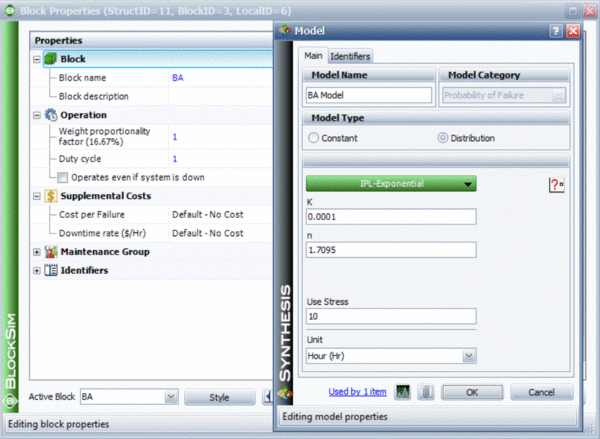
At this point, the parameters for the load sharing units have been computed and can be set, as shown in Figure "Load sharing parameters". (Note: when define the IPL-Exponential model, we just need to specify the value for K and n, the value for Use Stress is not a issue here, leave it as default number 10 or any number will be good.)
The next step is to set the weight proportionality factor. This factor defines the portion of the load that the particular item carries while operating, as well as the load that shifts to the remaining units upon failure of the item. To illustrate, assume three units (1, 2 and 3) are in a load sharing redundancy, represented in the fault tree diagram by a Load Sharing gate, with weight proportionality factors of 1, 2 and 3 respectively (and a 3-out-of-3 requirement).
- Unit 1 carries [math]\displaystyle{ \left( \tfrac{1}{1+2+3} \right)=0.166 }[/math] or 16.6% of the total load.
- Unit 2 carries [math]\displaystyle{ \left( \tfrac{2}{1+2+3} \right)=0.333 }[/math] or 33.3% of the total load.
- Unit 3 carries [math]\displaystyle{ \left( \tfrac{3}{1+2+3} \right)=0.50 }[/math] or 50% of the total load.
The actual load on each unit then becomes the product of the entire load defined for the gate multiplied by the portion carried by that unit. For example, if the load is 100 lbs, then the portion assigned to Unit 1 will be [math]\displaystyle{ 100\cdot 0.166=16.6 }[/math] lbs.
In the current example, all units share the same load; thus, they have equal weight proportionality factors. Because these factors are relative, if the same number is used for all three items then the results will be the same. For simplicity, we will set the factor equal to 1 for each item.
Once the properties have been specified in BlockSim, the reliability at 1000 hours can be determined. From the Analytical QCP, this is found to be 93.87%.


