Basic Statistical Background: Difference between revisions
Lisa Hacker (talk | contribs) No edit summary |
|||
| (28 intermediate revisions by 5 users not shown) | |||
| Line 1: | Line 1: | ||
{{template:LDABOOK|2|Basic Statistical Background}} | {{template:LDABOOK|2|Basic Statistical Background}} | ||
This section provides a brief elementary introduction to the most common and fundamental statistical equations and definitions used in reliability engineering and life data analysis. | |||
{{:Brief_Statistical_Background}} | |||
{{ | |||
Latest revision as of 09:16, 1 August 2012
This section provides a brief elementary introduction to the most common and fundamental statistical equations and definitions used in reliability engineering and life data analysis.
Random Variables

In general, most problems in reliability engineering deal with quantitative measures, such as the time-to-failure of a component, or qualitative measures, such as whether a component is defective or non-defective. We can then use a random variable [math]\displaystyle{ X\,\! }[/math] to denote these possible measures.
In the case of times-to-failure, our random variable [math]\displaystyle{ X\,\! }[/math] is the time-to-failure of the component and can take on an infinite number of possible values in a range from 0 to infinity (since we do not know the exact time a priori). Our component can be found failed at any time after time 0 (e.g., at 12 hours or at 100 hours and so forth), thus [math]\displaystyle{ X\,\! }[/math] can take on any value in this range. In this case, our random variable [math]\displaystyle{ X\,\! }[/math] is said to be a continuous random variable. In this reference, we will deal almost exclusively with continuous random variables.
In judging a component to be defective or non-defective, only two outcomes are possible. That is, [math]\displaystyle{ X\,\! }[/math] is a random variable that can take on one of only two values (let's say defective = 0 and non-defective = 1). In this case, the variable is said to be a discrete random variable.
The Probability Density Function and the Cumulative Distribution Function
The probability density function (pdf) and cumulative distribution function (cdf) are two of the most important statistical functions in reliability and are very closely related. When these functions are known, almost any other reliability measure of interest can be derived or obtained. We will now take a closer look at these functions and how they relate to other reliability measures, such as the reliability function and failure rate.
From probability and statistics, given a continuous random variable [math]\displaystyle{ X,\,\! }[/math] we denote:
- The probability density function, pdf, as [math]\displaystyle{ f(x)\,\! }[/math].
- The cumulative distribution function, cdf, as [math]\displaystyle{ F(x)\,\! }[/math].
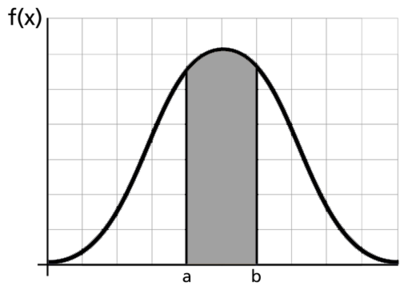
The pdf and cdf give a complete description of the probability distribution of a random variable. The following figure illustrates a pdf.

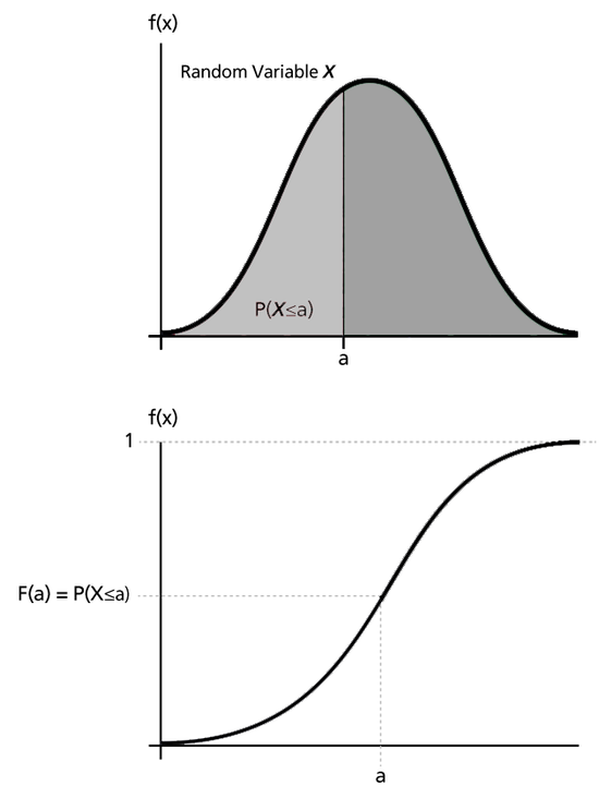
The next figures illustrate the pdf - cdf relationship.

If [math]\displaystyle{ X\,\! }[/math] is a continuous random variable, then the pdf of [math]\displaystyle{ X\,\! }[/math] is a function, [math]\displaystyle{ f(x)\,\! }[/math], such that for any two numbers, [math]\displaystyle{ a\,\! }[/math] and [math]\displaystyle{ b\,\! }[/math] with [math]\displaystyle{ a\le b\,\! }[/math] :
- [math]\displaystyle{ P(a\le X\le b)=\int_{a}^{b}f(x)dx\ \,\! }[/math]
That is, the probability that [math]\displaystyle{ X\,\! }[/math] takes on a value in the interval [math]\displaystyle{ [a,b]\,\! }[/math] is the area under the density function from [math]\displaystyle{ a\,\! }[/math] to [math]\displaystyle{ b,\,\! }[/math] as shown above. The pdf represents the relative frequency of failure times as a function of time.
The cdf is a function, [math]\displaystyle{ F(x)\,\! }[/math], of a random variable [math]\displaystyle{ X\,\! }[/math], and is defined for a number [math]\displaystyle{ x\,\! }[/math] by:
- [math]\displaystyle{ F(x)=P(X\le x)=\int_{0}^{x}f(s)ds\ \,\! }[/math]
That is, for a number [math]\displaystyle{ x\,\! }[/math], [math]\displaystyle{ F(x)\,\! }[/math] is the probability that the observed value of [math]\displaystyle{ X\,\! }[/math] will be at most [math]\displaystyle{ x\,\! }[/math]. The cdf represents the cumulative values of the pdf. That is, the value of a point on the curve of the cdf represents the area under the curve to the left of that point on the pdf. In reliability, the cdf is used to measure the probability that the item in question will fail before the associated time value, [math]\displaystyle{ t\,\! }[/math], and is also called unreliability.
Note that depending on the density function, denoted by [math]\displaystyle{ f(x)\,\! }[/math], the limits will vary based on the region over which the distribution is defined. For example, for the life distributions considered in this reference, with the exception of the normal distribution, this range would be [math]\displaystyle{ [0,+\infty ].\,\! }[/math]
Mathematical Relationship: pdf and cdf
The mathematical relationship between the pdf and cdf is given by:
- [math]\displaystyle{ F(x)=\int_{0}^{x}f(s)ds \,\! }[/math]
where [math]\displaystyle{ s\,\! }[/math] is a dummy integration variable.
Conversely:
- [math]\displaystyle{ f(x)=\frac{d(F(x))}{dx}\,\! }[/math]
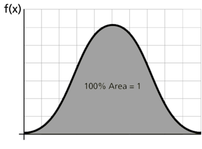
The cdf is the area under the probability density function up to a value of [math]\displaystyle{ x\,\! }[/math]. The total area under the pdf is always equal to 1, or mathematically:

- [math]\displaystyle{ \int_{-\infty}^{+\infty }f(x)dx=1\,\! }[/math]
The well-known normal (or Gaussian) distribution is an example of a probability density function. The pdf for this distribution is given by:
- [math]\displaystyle{ f(t)=\frac{1}{\sigma \sqrt{2\pi }}{{e}^{-\tfrac{1}{2}{{\left( \tfrac{t-\mu }{\sigma } \right)}^{2}}}}\,\! }[/math]
where [math]\displaystyle{ \mu \,\! }[/math] is the mean and [math]\displaystyle{ \sigma \,\! }[/math] is the standard deviation. The normal distribution has two parameters, [math]\displaystyle{ \mu \,\! }[/math] and [math]\displaystyle{ \sigma \,\! }[/math].
Another is the lognormal distribution, whose pdf is given by:
- [math]\displaystyle{ f(t)=\frac{1}{t\cdot {{\sigma }^{\prime }}\sqrt{2\pi }}{{e}^{-\tfrac{1}{2}{{\left( \tfrac{{{t}^{\prime }}-{{\mu }^{\prime }}}{{{\sigma }^{\prime }}} \right)}^{2}}}}\,\! }[/math]
where [math]\displaystyle{ {\mu }'\,\! }[/math] is the mean of the natural logarithms of the times-to-failure and [math]\displaystyle{ {\sigma }'\,\! }[/math] is the standard deviation of the natural logarithms of the times-to-failure. Again, this is a 2-parameter distribution.
Reliability Function
The reliability function can be derived using the previous definition of the cumulative distribution function, [math]\displaystyle{ F(x)=\int_{0}^{x}f(s)ds \,\! }[/math]. From our definition of the cdf, the probability of an event occurring by time [math]\displaystyle{ t\,\! }[/math] is given by:
- [math]\displaystyle{ F(t)=\int_{0}^{t}f(s)ds\ \,\! }[/math]
Or, one could equate this event to the probability of a unit failing by time [math]\displaystyle{ t\,\! }[/math].
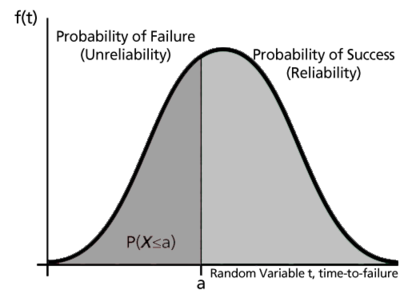
Since this function defines the probability of failure by a certain time, we could consider this the unreliability function. Subtracting this probability from 1 will give us the reliability function, one of the most important functions in life data analysis. The reliability function gives the probability of success of a unit undertaking a mission of a given time duration. The following figure illustrates this.

To show this mathematically, we first define the unreliability function, [math]\displaystyle{ Q(t)\,\! }[/math], which is the probability of failure, or the probability that our time-to-failure is in the region of 0 and [math]\displaystyle{ t\,\! }[/math]. This is the same as the cdf. So from [math]\displaystyle{ F(t)=\int_{0}^{t}f(s)ds\ \,\! }[/math]:
- [math]\displaystyle{ Q(t)=F(t)=\int_{0}^{t}f(s)ds\,\! }[/math]
Reliability and unreliability are the only two events being considered and they are mutually exclusive; hence, the sum of these probabilities is equal to unity.
Then:
- [math]\displaystyle{ \begin{align} Q(t)+R(t)= & 1 \\ R(t)= & 1-Q(t) \\ R(t)= & 1-\int_{0}^{t}f(s)ds \\ R(t)= & \int_{t}^{\infty }f(s)ds \end{align}\,\! }[/math]
Conversely:
- [math]\displaystyle{ f(t)=-\frac{d(R(t))}{dt}\,\! }[/math]
Conditional Reliability Function
Conditional reliability is the probability of successfully completing another mission following the successful completion of a previous mission. The time of the previous mission and the time for the mission to be undertaken must be taken into account for conditional reliability calculations. The conditional reliability function is given by:
- [math]\displaystyle{ R(t|T)=\frac{R(T+t)}{R(T)}\ \,\! }[/math]
Failure Rate Function
The failure rate function enables the determination of the number of failures occurring per unit time. Omitting the derivation, the failure rate is mathematically given as:
- [math]\displaystyle{ \lambda (t)=\frac{f(t)}{R(t)}\ \,\! }[/math]
This gives the instantaneous failure rate, also known as the hazard function. It is useful in characterizing the failure behavior of a component, determining maintenance crew allocation, planning for spares provisioning, etc. Failure rate is denoted as failures per unit time.
Mean Life (MTTF)
The mean life function, which provides a measure of the average time of operation to failure, is given by:
- [math]\displaystyle{ \overline{T}=m=\int_{0}^{\infty }t\cdot f(t)dt\,\! }[/math]
This is the expected or average time-to-failure and is denoted as the MTTF (Mean Time To Failure).
The MTTF, even though an index of reliability performance, does not give any information on the failure distribution of the component in question when dealing with most lifetime distributions. Because vastly different distributions can have identical means, it is unwise to use the MTTF as the sole measure of the reliability of a component.
Median Life
Median life,
[math]\displaystyle{ \tilde{T}\,\! }[/math],
is the value of the random variable that has exactly one-half of the area under the pdf to its left and one-half to its right.
It represents the centroid of the distribution.
The median is obtained by solving the following equation for [math]\displaystyle{ \breve{T}\,\! }[/math]. (For individual data, the median is the midpoint value.)
- [math]\displaystyle{ \int_{-\infty}^{{\breve{T}}}f(t)dt=0.5\ \,\! }[/math]
Modal Life (or Mode)
The modal life (or mode), [math]\displaystyle{ \tilde{T}\,\! }[/math], is the value of [math]\displaystyle{ T\,\! }[/math] that satisfies:
- [math]\displaystyle{ \frac{d\left[ f(t) \right]}{dt}=0\ \,\! }[/math]
For a continuous distribution, the mode is that value of [math]\displaystyle{ t\,\! }[/math] that corresponds to the maximum probability density (the value at which the pdf has its maximum value, or the peak of the curve).
Lifetime Distributions
A statistical distribution is fully described by its pdf. In the previous sections, we used the definition of the pdf to show how all other functions most commonly used in reliability engineering and life data analysis can be derived. The reliability function, failure rate function, mean time function, and median life function can be determined directly from the pdf definition, or [math]\displaystyle{ f(t)\,\! }[/math]. Different distributions exist, such as the normal (Gaussian), exponential, Weibull, etc., and each has a predefined form of [math]\displaystyle{ f(t)\,\! }[/math] that can be found in many references. In fact, there are certain references that are devoted exclusively to different types of statistical distributions. These distributions were formulated by statisticians, mathematicians and engineers to mathematically model or represent certain behavior. For example, the Weibull distribution was formulated by Waloddi Weibull and thus it bears his name. Some distributions tend to better represent life data and are most commonly called "lifetime distributions".
A more detailed introduction to this topic is presented in Life Distributions.
