Example: Gumbel Distribution: Difference between revisions
Chris Kahn (talk | contribs) No edit summary |
Chris Kahn (talk | contribs) No edit summary |
||
| Line 1: | Line 1: | ||
{| class="FCK__ShowTableBorders" border="0" cellspacing="0" cellpadding="0" align="center"; style="width:100%;" | {| class="FCK__ShowTableBorders" border="0" cellspacing="0" cellpadding="0" align="center"; style="width:100%;" | ||
|- | |- | ||
| valign="middle" align="left" bgcolor=EEEDF7|[[Image: | | valign="middle" align="left" bgcolor=EEEDF7|[[Image:Weibull_Examples_Banner.png|400px|center]] | ||
|} | |} | ||
<br> | <br> | ||
Revision as of 09:31, 26 July 2012
Verify using Monte Carlo simulation that if [math]\displaystyle{ {{t}_{i}} }[/math] follows a Weibull distribution with [math]\displaystyle{ \beta }[/math] and [math]\displaystyle{ \eta }[/math] , then the [math]\displaystyle{ Ln({{t}_{i}}) }[/math] follows a Gumbel distribution with [math]\displaystyle{ \mu =\ln (\eta ) }[/math] and [math]\displaystyle{ \sigma =1/\beta. }[/math]
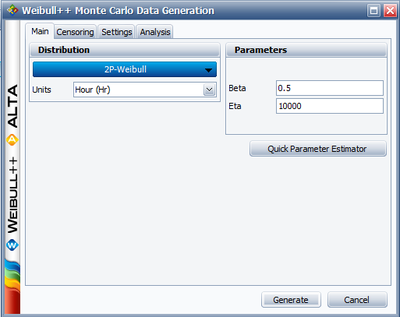
Let us assume that [math]\displaystyle{ {{t}_{i}} }[/math] follows a Weibull distribution with [math]\displaystyle{ \beta =0.5 }[/math] and [math]\displaystyle{ \eta =10000. }[/math] The Monte Carlo simulation tool in Weibull++ can be used to generate a set of random numbers that follow a Weibull distribution with the specified parameters.
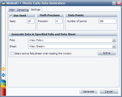
Other simulation settings are:
After obtaining the random time values [math]\displaystyle{ {{t}_{i}} }[/math] , insert a new data sheet into the folio. In this sheet enter the [math]\displaystyle{ Ln({{t}_{i}}) }[/math] values using the LN function and referring to the cells in the sheet that contains the [math]\displaystyle{ {{t}_{i}} }[/math] values. Delete any negative values, if there are any (since Weibull++ expects all time values to be positive). Calculate the parameters of the Gumbel distribution that fits the [math]\displaystyle{ Ln({{t}_{i}}) }[/math] values.
Using maximum likelihood as the analysis method, the estimated parameters are:
- [math]\displaystyle{ \begin{align} & \hat{\mu }= & 9.3816 \\ & \hat{\sigma }= & 1.9717 \end{align} }[/math]
Since [math]\displaystyle{ \ln (\eta )= }[/math] 9.2103 ( [math]\displaystyle{ \simeq 9.3816 }[/math] ) and [math]\displaystyle{ 1/\beta =2 }[/math] [math]\displaystyle{ (\simeq 1.9717), }[/math] then this simulation verifies that [math]\displaystyle{ Ln({{t}_{i}}) }[/math] follows a Gumbel distribution with [math]\displaystyle{ \mu =\ln (\eta ) }[/math] and [math]\displaystyle{ \delta =1/\beta . }[/math]
Note: This example illustrates a property of the Gumbel distribution; it is not meant to be a formal proof.


