Template:Example: Warranty Analysis Nevada Format Example: Difference between revisions
No edit summary |
No edit summary |
||
| Line 60: | Line 60: | ||
Even though this step is not required for the analysis, the data can also be transferred to a Weibull++ data sheet for illustrative purposes or for ancillary analysis. This can be done by clicking the Transfer Life Data to New Folio button: | Even though this step is not required for the analysis, the data can also be transferred to a Weibull++ data sheet for illustrative purposes or for ancillary analysis. This can be done by clicking the Transfer Life Data to New Folio button: | ||
[[Image:transferdata2folio.png|center ]] | [[Image:transferdata2folio.png|center|250px ]] | ||
<math></math> | <math></math> | ||
Revision as of 22:09, 25 April 2012
Warranty Analysis Nevada Format Example
A company keeps track of its shipments and warranty returns on a month-by-month basis. The data format that the company uses is the Nevada format. Following is a table for shipments in June, July, and August, and the warranty returns through September:
| RETURNS | ||||
| SHIP | Jul. 2010 | Aug. 2010 | Sep. 2010 | |
| Jun. 2010 | 100 | 3 | 3 | 5 |
| Jul. 2010 | 140 | - | 2 | 4 |
| Aug. 2010 | 150 | - | - | 4 |
Convert this information to life data, and determine the parameters for a two-parameter Weibull distribution.
Solution
We will examine the data month by month. In June 100 units were sold, and in July three of these units were returned. This gives three failures at one month for the June shipment, which we will denote as [math]\displaystyle{ {{F}_{JUN,1}}=3 }[/math] . Likewise, three failures occurred in August and five occurred in September for this shipment, or [math]\displaystyle{ {{F}_{JUN,2}}=3 }[/math] and [math]\displaystyle{ {{F}_{JUN,3}}=5. }[/math] Consequently, at the end of our three-month analysis period, there were a total of 11 failures for the 100 units shipped in June. This means that 89 units are presumably still operating, and can be considered suspensions at three months, or [math]\displaystyle{ {{S}_{JUN,3}}=89 }[/math] . For the shipment of 140 in July, two were returned the following month, or [math]\displaystyle{ {{F}_{JUL,1}}=2 }[/math] , and four more were returned the month after that, or [math]\displaystyle{ {{F}_{JUL,2}}=4. }[/math] After two months, there are 134 ( [math]\displaystyle{ 140-2-4=134 }[/math] ) units from the July shipment still operating, or [math]\displaystyle{ {{S}_{JUL,2}}=134 }[/math]. For the final shipment of 150 in August, four fail in September, or [math]\displaystyle{ {{F}_{AUG,1}}=4 }[/math], with the remaining 146 units being suspensions at one month, or [math]\displaystyle{ {{S}_{AUG,1}}=146 }[/math] .
It is now a simple matter to add up the number of failures for 1, 2, and 3 months, then add the suspensions to get our reliability data set:
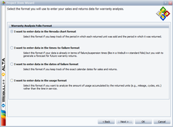
To perform this analysis using the Warranty Analysis tool in Weibull++, create a Warranty Analysis Folio and choose I want to enter data inNevada format in the Project Wizard.
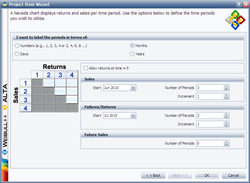
The next window allows you to specify the time units used. For this example select Months under I want to use the following unit type for each period and enter the Start month and Number of Periods and Increment number for the sales data and failure/return data as follows:
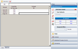
The sales data are entered as follows:
The return data are entered as follows:
The data can now be analyzed. Select two-parameter Weibull as the distribution type and MLE as the analysis method and click the Calculate button. The estimated parameters are [math]\displaystyle{ \widehat{\beta }=2.49 }[/math] and [math]\displaystyle{ \widehat{\eta }=6.70. }[/math]
Even though this step is not required for the analysis, the data can also be transferred to a Weibull++ data sheet for illustrative purposes or for ancillary analysis. This can be done by clicking the Transfer Life Data to New Folio button:
[math]\displaystyle{ }[/math]
or choosing this option under the Data menu.
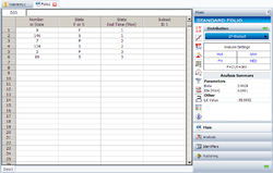
The equivalent Times-to-failure folio is as follows:


