Template:Example: Generalized Gamma Distribution Example: Difference between revisions
No edit summary |
No edit summary |
||
| Line 29: | Line 29: | ||
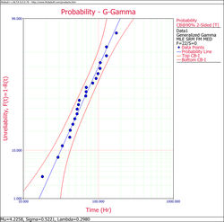
In Weibull++ the generalized gamma probability is plotted on gamma probability paper, as shown next. | In Weibull++ the generalized gamma probability is plotted on gamma probability paper, as shown next. | ||
[[Image:GGamma Example 1 Plot.png|thumb|center| | [[Image:GGamma Example 1 Plot.png|thumb|center|250px| ]] | ||
It is important to also note that as in the case of the mixed Weibull distribution, in the case of regression analysis, using a generalized gamma model, the choice of regression axis, i.e. <math>RRX</math> or <math>RRY,</math> is of no consequence since non-linear regression is utilized. | It is important to also note that as in the case of the mixed Weibull distribution, in the case of regression analysis, using a generalized gamma model, the choice of regression axis, i.e. <math>RRX</math> or <math>RRY,</math> is of no consequence since non-linear regression is utilized. | ||
Revision as of 21:56, 25 April 2012
A Generalized Gamma Distribution Example Example: Generalized Gamma Distribution Example The following data set represents revolutions-to-failure (in millions) for 23 ball bearings in a fatigue test [21].
- [math]\displaystyle{ \begin{array}{*{35}{l}} \text{17}\text{.88} & \text{28}\text{.92} & \text{33} & \text{41}\text{.52} & \text{42}\text{.12} & \text{45}\text{.6} & \text{48}\text{.4} & \text{51}\text{.84} & \text{51}\text{.96} & \text{54}\text{.12} \\ \text{55}\text{.56} & \text{67}\text{.8} & \text{68}\text{.64} & \text{68}\text{.64} & \text{68}\text{.88} & \text{84}\text{.12} & \text{93}\text{.12} & \text{98}\text{.64} & \text{105}\text{.12} & \text{105}\text{.84} \\ \text{127}\text{.92} & \text{128}\text{.04} & \text{173}\text{.4} & {} & {} & {} & {} & {} & {} & {} \\ \end{array} }[/math]
When the generalized gamma distribution is fitted to this data using MLE, the following values for parameters are obtained:
- [math]\displaystyle{ \begin{align} & \widehat{\mu }= & 4.23064 \\ & \widehat{\sigma }= & 0.509982 \\ & \widehat{\lambda }= & 0.307639 \end{align} }[/math]
Note that for this data, the generalized gamma offers a compromise between the Weibull [math]\displaystyle{ (\lambda =1), }[/math] and the lognormal [math]\displaystyle{ (\lambda =0) }[/math] distributions. The value of [math]\displaystyle{ \lambda }[/math] indicates that the lognormal distribution is better supported by the data. A better assessment, however, can be made by looking at the confidence bounds on [math]\displaystyle{ \lambda . }[/math] For example, the 90% two-sided confidence bounds are:
- [math]\displaystyle{ \begin{align} & {{\lambda }_{u}}= & -0.592087 \\ & {{\lambda }_{u}}= & 1.20736 \end{align} }[/math]
It can be then concluded that both distributions (i.e. Weibull and lognormal) are well supported by the data, with the lognormal being the ,better supported of the two. In Weibull++ the generalized gamma probability is plotted on gamma probability paper, as shown next.
It is important to also note that as in the case of the mixed Weibull distribution, in the case of regression analysis, using a generalized gamma model, the choice of regression axis, i.e. [math]\displaystyle{ RRX }[/math] or [math]\displaystyle{ RRY, }[/math] is of no consequence since non-linear regression is utilized.
