Template:Example: Published 3P Weibull Distribution Probability Plot Example: Difference between revisions
No edit summary |
No edit summary |
||
| Line 23: | Line 23: | ||
[[Image:Weibull Distribution Example 19 Plot.png|center| | [[Image:Weibull Distribution Example 19 Plot.png|center|250px]] | ||
Revision as of 18:26, 25 April 2012
Published 3P Weibull Distribution Probability Plot Example
From Dimitri Kececioglu, Reliability & Life Testing Handbook, Page 406. [20].
Estimate the parameters for three-parameter Weibull, for a sample of ten units all tested to failure. The times-to-failure were recorded at 200; 370; 500; 620; 730; 840; 950; 1,050; 1,160; and 1,400 hours.
Published Results:
Published results (using probability plotting):
Computed Results in Weibull++
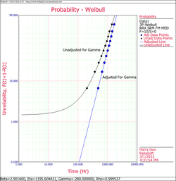
Weibull++ computed parameters for rank regression on X are:
The small difference between the published results and the ones obtained from Weibull++ are due to the difference in the estimation method. In the publication the parameters were estimated using probability plotting (i.e. the fitted line was "eye-balled"). In Weibull++, the parameters were estimated using non-linear regression (a more accurate, mathematically fitted line). Note that γ in this example is negative. This means that the unadjusted for γ line is concave up, as shown next.


