Template:Example: MLE for Exponential Distribution: Difference between revisions
No edit summary |
No edit summary |
||
| Line 22: | Line 22: | ||
Using Weibull++: | Using Weibull++: | ||
[[Image:Exponential Distribution Example 4 Data.png|thumb|center| | [[Image:Exponential Distribution Example 4 Data.png|thumb|center|250px|]] | ||
The probability plot is: | The probability plot is: | ||
[[Image:Exponential Distribution Example 4 Plot.png|thumb|center| | [[Image:Exponential Distribution Example 4 Plot.png|thumb|center|250px|]] | ||
Revision as of 17:55, 25 April 2012
MLE for Exponential Distribution
Using the data of Example 2 and assuming a two-parameter exponential distribution, estimate the parameters using the MLE method.
Solution
In this example we have complete data only. The partial derivative of the log-likelihood function, [math]\displaystyle{ \Lambda , }[/math] is given by:
- [math]\displaystyle{ \frac{\partial \Lambda }{\partial \lambda }=\underset{i=1}{\overset{{{F}_{e}}}{\mathop \sum }}\,\left[ \frac{1}{\lambda }-\left( {{T}_{i}}-\gamma \right) \right]=\underset{i=1}{\overset{14}{\mathop \sum }}\,\left[ \frac{1}{\lambda }-\left( {{T}_{i}}-\gamma \right) \right]=0 }[/math]
Complete descriptions of the partial derivatives can be found in Appendix. Recall that when using the MLE method for the exponential distribution, the value of [math]\displaystyle{ \gamma }[/math] is equal to that of the first failure time. The first failure occurred at 5 hours, thus [math]\displaystyle{ \gamma =5 }[/math] hours[math]\displaystyle{ . }[/math] Substituting the values for [math]\displaystyle{ T }[/math] and [math]\displaystyle{ \gamma }[/math] we get:
- [math]\displaystyle{ \frac{14}{\hat{\lambda }}=560 }[/math]
or:
- [math]\displaystyle{ \hat{\lambda }=0.025\text{ failures/hour}. }[/math]
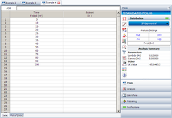
Using Weibull++:
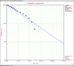
The probability plot is:

