Template:Example: Weibull Distribution Example-Demonstrate Reliability: Difference between revisions
Lisa Hacker (talk | contribs) |
Lisa Hacker (talk | contribs) No edit summary |
||
| Line 11: | Line 11: | ||
<br> | <br> | ||
<center><math>R={{e}^{-{{(t/\eta )}^{\beta }}}}</math></center> | |||
<br> | <br> | ||
| Line 19: | Line 19: | ||
<br> | <br> | ||
<center><math>\eta =\frac{{{t}_{DEMO}}}{{{(-\text{ln}({{R}_{DEMO}}))}^{\tfrac{1}{\beta }}}}</math></center> | |||
<br> | <br> | ||
| Line 27: | Line 27: | ||
<br> | <br> | ||
<center><math>\eta =\frac{100}{{{(-\text{ln}(0.9))}^{\tfrac{1}{1.5}}}}=448.3</math></center> | |||
<br> | <br> | ||
Next, the value of | Next, the value of <math>{{R}_{TEST}}</math> is calculated by: | ||
<br> | <br> | ||
<center><math>{{R}_{TEST}}={{e}^{-{{({{t}_{TEST}}/\eta )}^{\beta }}}}={{e}^{-{{(48/448.3)}^{1.5}}}}=0.966=96.6%</math></center> | |||
<br> | <br> | ||
| Line 43: | Line 43: | ||
<br> | <br> | ||
<center><math>1-C.L.=\underset{i=0}{\overset{f}{\mathop \sum }}\,\frac{n!}{i!\cdot (n-i)!}\cdot {{(1-{{e}^{-{{({{t}_{TEST}}/\eta )}^{\beta }}}})}^{i}}\cdot {{({{e}^{-{{({{t}_{TEST}}/\eta )}^{\beta }}}})}^{(n-i)}}</math></center> | |||
<br> | <br> | ||
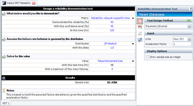
The values of <math>CL</math>, <math>{{t}_{TEST}}</math>, <math>\beta </math>, <math>f</math> and <math>\eta </math> have already been calculated or specified, so it merely remains to solve the equation for <math>n</math>. | The values of <math>CL</math>, <math>{{t}_{TEST}}</math>, <math>\beta </math>, <math>f</math> and <math>\eta </math> have already been calculated or specified, so it merely remains to solve the equation for <math>n</math>. This value is <math>n=85.4994</math>, or <math>n=86</math> units, since the fractional value must be rounded up to the next integer value. This example solved in Weibull++ is shown next. | ||
<br> | <br> | ||
| Line 57: | Line 57: | ||
'''Determining Time for Available Units''' | '''Determining Time for Available Units''' | ||
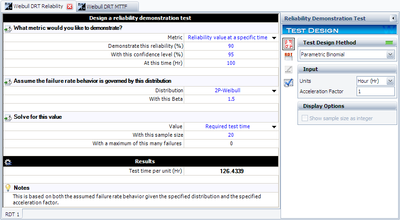
In this case, we will assume that we have 20 units to test, <math>n=20</math>, and must determine the test time, <math>{{t}_{TEST}}</math>. | In this case, we will assume that we have 20 units to test, <math>n=20</math>, and must determine the test time, <math>{{t}_{TEST}}</math>. We have already determined the value of the scale parameter, <math>\eta </math>, in the previous example. Since we know the values of <math>n</math>, <math>CL</math>, <math>f</math>, <math>\eta </math> and <math>\beta </math>, it remains to solve the binomial equation with the Weibull distribution for <math>{{t}_{TEST}}</math>. This value is <math>{{t}_{TEST}}=126.4339</math> hours. This example solved in Weibull++ is shown next. | ||
<br> | <br> | ||
[[Image:RDT Weibull Demonstrate Reliability Test Time.png|thumb|center|400px ]] | [[Image:RDT Weibull Demonstrate Reliability Test Time.png|thumb|center|400px ]] | ||
Revision as of 23:34, 29 March 2012
Weibull Distribution Example - Demonstrate Reliability
In this example, we will design a test to demonstrate a reliability of 90% at [math]\displaystyle{ t=100 }[/math] hours, with a 95% confidence. We will assume a Weibull distribution with a shape parameter [math]\displaystyle{ \beta =1.5 }[/math]. No failures will be allowed on this test, or [math]\displaystyle{ f=0 }[/math].
Determining Units for Available Time
In the above scenario, we know that we have the testing facilities available for [math]\displaystyle{ t=48 }[/math] hours. We must now determine the number of units to test for this amount of time with no failures in order to have demonstrated our reliability goal. The first step is to determine the Weibull scale parameter, [math]\displaystyle{ \eta }[/math]. The Weibull reliability equation is:
This can be rewritten as:
Since we know the values of [math]\displaystyle{ {{t}_{DEMO}} }[/math], [math]\displaystyle{ {{R}_{DEMO}} }[/math] and [math]\displaystyle{ \beta }[/math], we can substitute these in the equation and solve for [math]\displaystyle{ \eta }[/math]:
Next, the value of [math]\displaystyle{ {{R}_{TEST}} }[/math] is calculated by:
The last step is to substitute the appropriate values into the cumulative binomial equation, which for the Weibull distribution appears as:
The values of [math]\displaystyle{ CL }[/math], [math]\displaystyle{ {{t}_{TEST}} }[/math], [math]\displaystyle{ \beta }[/math], [math]\displaystyle{ f }[/math] and [math]\displaystyle{ \eta }[/math] have already been calculated or specified, so it merely remains to solve the equation for [math]\displaystyle{ n }[/math]. This value is [math]\displaystyle{ n=85.4994 }[/math], or [math]\displaystyle{ n=86 }[/math] units, since the fractional value must be rounded up to the next integer value. This example solved in Weibull++ is shown next.
Determining Time for Available Units
In this case, we will assume that we have 20 units to test, [math]\displaystyle{ n=20 }[/math], and must determine the test time, [math]\displaystyle{ {{t}_{TEST}} }[/math]. We have already determined the value of the scale parameter, [math]\displaystyle{ \eta }[/math], in the previous example. Since we know the values of [math]\displaystyle{ n }[/math], [math]\displaystyle{ CL }[/math], [math]\displaystyle{ f }[/math], [math]\displaystyle{ \eta }[/math] and [math]\displaystyle{ \beta }[/math], it remains to solve the binomial equation with the Weibull distribution for [math]\displaystyle{ {{t}_{TEST}} }[/math]. This value is [math]\displaystyle{ {{t}_{TEST}}=126.4339 }[/math] hours. This example solved in Weibull++ is shown next.

