Template:Example: Test Design Using Expected Failure Times Plot

Test Design Using Expected Failure Times Plot

Four units were allocated for a reliability test. The test engineers want to know how long the test will last if all the units are tested to failure. Based on previous experiments, they assume the underlying failure distribution is a Weibull distribution with [math]\displaystyle{ \beta }[/math] = 2 and [math]\displaystyle{ \eta }[/math] = 500.

Solution

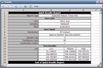
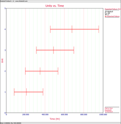
The expected failure time with 80% 2-sided confidence bounds are given below.

From the above results, we can see the upper bound of the last failure is about 955 hours. Therefore, the test probably will last for around 955 hours.

As we know, with four samples, the median rank for the second failure is 0.385728. Using this value and the assumed Weibull distribution, the median value of the failure time of the 2nd failure is calculated as:

[math]\displaystyle{ \begin{align} & Q=1-{{e}^{{{\left( \frac{t}{\eta } \right)}^{\beta }}}}\Rightarrow \\ & \ln (1-Q)={{\left( \frac{t}{\eta } \right)}^{\beta }} \\ & \Rightarrow t=\text{349.04}\\ \end{align} }[/math]

Its bounds and other failure times can be calculated in a similar way.