Template:Example: 2 Parameter Exponential Distribution RRX

2 Parameter Exponential Distribution RRX

Using the data of Example 2 and assuming a two-parameter exponential distribution, estimate the parameters and determine the correlation coefficient estimate, [math]\displaystyle{ \hat{\rho } }[/math], using rank regression on X.

Solution

The Table constructed in Example 2 applies to this example also. Using the values from this table, we get:

[math]\displaystyle{ \begin{align} \hat{b}= & \frac{\underset{i=1}{\overset{14}{\mathop{\sum }}}\,{{t}_{i}}{{y}_{i}}-\tfrac{\underset{i=1}{\overset{14}{\mathop{\sum }}}\,{{t}_{i}}\underset{i=1}{\overset{14}{\mathop{\sum }}}\,{{y}_{i}}}{14}}{\underset{i=1}{\overset{14}{\mathop{\sum }}}\,y_{i}^{2}-\tfrac{{{\left( \underset{i=1}{\overset{14}{\mathop{\sum }}}\,{{y}_{i}} \right)}^{2}}}{14}} \\ \\ \hat{b}= & \frac{-927.4899-(630)(-13.2315)/14}{22.1148-{{(-13.2315)}^{2}}/14} \end{align} }[/math]

or:

[math]\displaystyle{ \hat{b}=-34.5563 }[/math]

and:

[math]\displaystyle{ \hat{a}=\overline{x}-\hat{b}\overline{y}=\frac{\underset{i=1}{\overset{14}{\mathop{\sum }}}\,{{t}_{i}}}{14}-\hat{b}\frac{\underset{i=1}{\overset{14}{\mathop{\sum }}}\,{{y}_{i}}}{14} }[/math]

or:

[math]\displaystyle{ \hat{a}=\frac{630}{14}-(-34.5563)\frac{(-13.2315)}{14}=12.3406 }[/math]

Therefore:

[math]\displaystyle{ \hat{\lambda }=-\frac{1}{\hat{b}}=-\frac{1}{(-34.5563)}=0.0289\text{ failures/hour} }[/math]

and:

[math]\displaystyle{ \hat{\gamma }=\hat{a}=12.3406 }[/math]

The correlation coefficient is found to be:

[math]\displaystyle{ \hat{\rho }=-0.9679 }[/math]

Note that the equation for regression on Y is not necessarily the same as that for the regression on X. The only time when the two regression methods yield identical results is when the data lie perfectly on a line. If this were the case, the correlation coefficient would be [math]\displaystyle{ -1 }[/math]. The negative value of the correlation coefficient is due to the fact that the slope of the exponential probability plot is negative.

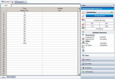
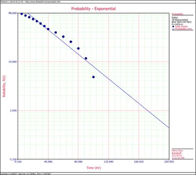
This example can be repeated using Weibull++, choosing two-parameter exponential and rank regression on X (RRX) methods for analysis, as shown below. The estimated parameters and the correlation coefficient using Weibull++ were found to be:

[math]\displaystyle{ \begin{array}{*{35}{l}} \hat{\lambda }= &0.0289 \text{failures/hour} \\ \hat{\gamma}= & 12.3395 \text{hours} \\ \hat{\rho} = &-0.9679 \\ \end{array} }[/math]

The probability plot can be obtained simply by clicking the Plot icon.