Template:Maximum Likelihood Estimation for Exponential Distribution

Maximum Likelihood Estimation for Exponential Distribution

As outlined in Chapter 4, maximum likelihood estimation works by developing a likelihood function based on the available data and finding the values of the parameter estimates that maximize the likelihood function. This can be achieved by using iterative methods to determine the parameter estimate values that maximize the likelihood function. This can be rather difficult and time-consuming, particularly when dealing with the three-parameter distribution. Another method of finding the parameter estimates involves taking the partial derivatives of the likelihood equation with respect to the parameters, setting the resulting equations equal to zero, and solving simultaneously to determine the values of the parameter estimates. The log-likelihood functions and associated partial derivatives used to determine maximum likelihood estimates for the exponential distribution are covered in Appendix.

Example 4: MLE for Exponential Distribution

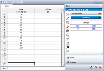
Using the data of Example 2 and assuming a two-parameter exponential distribution, estimate the parameters using the MLE method.

Solution to Example 4

In this example we have complete data only. The partial derivative of the log-likelihood function, [math]\displaystyle{ \Lambda , }[/math] is given by:

[math]\displaystyle{ \frac{\partial \Lambda }{\partial \lambda }=\underset{i=1}{\overset{{{F}_{e}}}{\mathop \sum }}\,\left[ \frac{1}{\lambda }-\left( {{T}_{i}}-\gamma \right) \right]=\underset{i=1}{\overset{14}{\mathop \sum }}\,\left[ \frac{1}{\lambda }-\left( {{T}_{i}}-\gamma \right) \right]=0 }[/math]

Complete descriptions of the partial derivatives can be found in Appendix. Recall that when using the MLE method for the exponential distribution, the value of [math]\displaystyle{ \gamma }[/math] is equal to that of the first failure time. The first failure occurred at 5 hours, thus [math]\displaystyle{ \gamma =5 }[/math] hours[math]\displaystyle{ . }[/math] Substituting the values for [math]\displaystyle{ T }[/math] and [math]\displaystyle{ \gamma }[/math] we get:

[math]\displaystyle{ \frac{14}{\hat{\lambda }}=560 }[/math]

or:

[math]\displaystyle{ \hat{\lambda }=0.025\text{ failures/hour}. }[/math]

Using Weibull++:

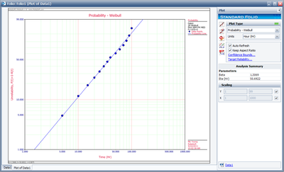
The probability plot is: