Template:Warranty analysis usage example

Warranty Usage Example

Suppose that an automotive manufacturer collects the warranty returns and sales data given in section 12.3.1.4 for a particular part in a given region. Convert this information to life data and fit a suitable distribution to it.

Solution

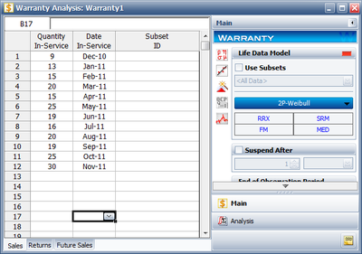
To perform this analysis using the Warranty Analysis tool in Weibull++, create a Warranty Analysis Folio and choose I want to enter data in usage format in the Project Wizard. The sales data are entered as follows:

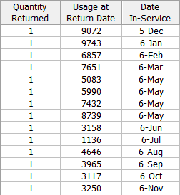
The return data (accumulated mileage at time of failure and the date the failed unit was put in-service ( [math]\displaystyle{ DIS }[/math] )) is shown in the next figure.

The above figure also shows the calculation End Date ( [math]\displaystyle{ ED }[/math] ), which can be set on the Analysis page of the Control Panel. In this example, the warranty data were collected until 12/1/2006.

The user has the option to input either a constant value that describes an average of usage or a distribution with intervals to be considered in the analysis. In this example, the manufacturer has been documenting the mileage accumulation per year for this type of product across the customer base in comparable regions for many years. The yearly usage has been determined to follow a lognormal distribution with [math]\displaystyle{ {{\mu }_{T\prime }}=9.38 }[/math] , [math]\displaystyle{ {{\sigma }_{T\prime }}=0.085 }[/math] . Graphically, the distribution looks as follows.

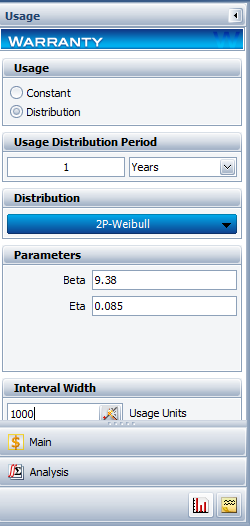
The usage distribution is specified on the Usage page of the Control Panel, as shown next.

[math]\displaystyle{ }[/math]

Note that the Interval Width was defined to be 1000 miles (as seen in the above figure). This interval facilitates the calculations of mileage usage for the suspensions in the data set.

In addition to 14 failures, the data set contains 212 suspensions spread according to the defined usage distribution. Note that due to rounding-off in the calculation, only 208 of these suspensions are ultimately allocated. This data set contains 12 groups of suspensions that have the same age. To illustrate the analysis procedure explained above, let us use one suspension group, the first group. The first group contains 9 units that went in service on a given date; 1 unit failed from that batch. Therefore, 8 suspensions have survived from December 2005 until the beginning of December 2006, a total of 12 months. The calculations are summarized as follows.

The two columns on the right constitute the calculated suspension data (number of suspensions and their usage) for the first group. The calculation in the above table is then repeated for each of the remaining 11 suspension groups in the data set. We then add the resulting data and the failure data and proceed with estimating a failure distribution model.

The data set that is used to perform the estimation of the failure distribution model can be extracted and displayed by selecting Transfer Life Data to New Folio from the Data menu. The failures and suspensions data set, as presented in the Standard Folio, is partially shown next. (Note that the Folio contains 66 rows.)

The entered sales and return data set, the usage distribution and the interval width in the Warranty Folio can be used to derive a failure distribution. The manufacturer assumes that the observed failures are typically modeled by a lognormal distribution. The parameters of the distribution are estimated (by clicking on the Calculate button) to be:

[math]\displaystyle{ \begin{align} & {{\mu }_{T\prime }}= & 10.4747 \\ & {{\sigma }_{T\prime }}= & 1.1159 \end{align} }[/math]

The reliability plot (with mileage being the random variable driving reliability), along with the 90% confidence bounds on reliability, is shown next.