Template:Logistic (reliability growth model)

Logistic

The Logistic reliability growth model has an S-shaped curve and is given by [3]:

where [math]\displaystyle{ b }[/math] and [math]\displaystyle{ k }[/math] are parameters. Similar to the analysis given for the Gompertz curve (Chapter 7), the following may be concluded:

1) The point of inflection is given by:

[math]\displaystyle{ {{T}_{i}}=\frac{\ln (b)}{k} }[/math]

2) When [math]\displaystyle{ b\gt 1 }[/math] then [math]\displaystyle{ {{T}_{i}}\gt 0 }[/math] and an S-shaped curve will be generated. However, w[math]\displaystyle{ % }[/math]hen [math]\displaystyle{ 0\lt b\le 1 }[/math] then [math]\displaystyle{ {{T}_{i}}\le 0 }[/math] and the Logistic reliability growth model will not be described by an S-shaped curve.

3) The value of [math]\displaystyle{ R }[/math] is equal to 0.5 at the inflection point.

The Logistic reliability growth model has an S-shaped curve and is given by Kececioglu [3]:

[math]\displaystyle{ R = \frac{1}{1+be^{-kt}}, b \gt 0, k \gt 0, T \simeq 0 }[/math]

where [math]\displaystyle{ b\,\! }[/math] and [math]\displaystyle{ k\,\! }[/math] are parameters. Similar to the analysis given for the Gompertz curve, the following may be concluded:

1. The point of inflection is given by:

   [math]\displaystyle{ {{T}_{i}}=\frac{\ln (b)}{k}\,\! }[/math]

2. When [math]\displaystyle{ b\gt 1\,\! }[/math], then [math]\displaystyle{ {{T}_{i}}\gt 0\,\! }[/math] and an S-shaped curve will be generated. However, when [math]\displaystyle{ 0\lt b\le 1\,\! }[/math] , then [math]\displaystyle{ {{T}_{i}}\le 0\,\! }[/math] and the Logistic reliability growth model will not be described by an S-shaped curve.
3. The value of [math]\displaystyle{ R\,\! }[/math] is equal to 0.5 at the inflection point.

Parameter Estimation

In this section, we will demonstrate the parameter estimation method for the Logistic model using three examples for different types of data.

Example: Logistic for Reliability Data

Using the reliability growth data given in the table below, do the following:

1. Find a Gompertz curve that represents the data and plot it with the raw data.
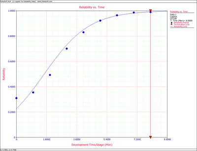
2. Find a Logistic reliability growth curve that represents the data and plot it with the raw data.

Development Time vs. Observed Reliability data and Predicted Reliabilities

Time, months	Raw Data Reliability (%)	Gompertz Reliability (%)	Logistic Reliablity (%)
0	31.00	24.85	22.73
1	35.50	38.48	38.14
2	49.30	51.95	56.37
3	70.10	63.82	73.02
4	83.00	73.49	85.01
5	92.20	80.95	92.24
6	96.40	86.51	96.14
7	98.60	90.54	98.12
8	99.00	93.41	99.09

Solution

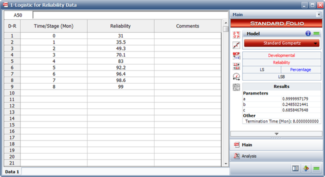
1. The figure below shows the entered data and the estimated parameters using the standard Gompertz model.
   

   Therefore:

   [math]\displaystyle{ \begin{align} & \widehat{a}= & 0.9999 \\ & \widehat{b}= & 0.2485 \\ & \widehat{c}= & 0.6858 \end{align}\,\! }[/math]

   [math]\displaystyle{ R=(0.9999){{(0.2485)}^{{{0.6858}^{T}}}}\,\! }[/math]

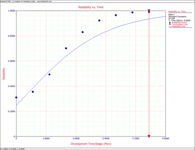
   The values of the predicted reliabilities are plotted in the figure below.

   

   Notice how the standard Gompertz model is not really capable of handling the S-shaped characteristics of this data.

2. The least squares estimators of the Logistic growth curve parameters are given by Crow [9]: where:

   [math]\displaystyle{ \begin{align} {{{\hat{b}}}_{1}}= & \frac{\underset{i=0}{\overset{N-1}{\mathop{\sum }}}\,{{T}_{i}}{{Y}_{i}}-N\cdot \bar{T}\cdot \bar{Y}}{\underset{i=0}{\overset{N-1}{\mathop{\sum }}}\,T_{i}^{2}-N\cdot {{{\bar{T}}}^{2}}} \\ \\ {{{\hat{b}}}_{0}}= & \bar{Y}-{{{\hat{b}}}_{1}}\bar{T} \\ \\ {{Y}_{i}}= & \ln \left( \frac{1}{{{R}_{i}}}-1 \right) \\ \\ \bar{Y}= & \frac{1}{N}\underset{i=0}{\overset{N-1}{\mathop \sum }}\,{{Y}_{i}} \end{align}\,\! }[/math]

   In this example [math]\displaystyle{ N=9\,\! }[/math], which gives:

   [math]\displaystyle{ \begin{align} \overline{Y}&=\frac{1}{9}\sum_{i=0}^{8}ln\left (\frac{1}{R_{i}}-1 \right ) \\ &= -1.7355 \\ \\ \overline{T}&=\frac{1}{9}\sum_{i=0}^{8}T_{i} = 4 \\ \sum_{i=0}^{8}T_{i}^{2} &= 204 \\ \sum_{i=0}^{8}T_{i}Y_{i} &= -106.8630 \end{align}\,\! }[/math]

   From the equations for [math]\displaystyle{ b_{i}\,\! }[/math] and [math]\displaystyle{ \hat{b_{0}}\,\! }[/math]:

   [math]\displaystyle{ \begin{align} \hat{b_{1}} &= \frac{-106.8630 - 9(4)(-1.7355)}{204-9(4)_{2}} \\ & = 0.7398 \\ \hat{b_{0}} &= -1.7355 - (-0.7398)(4)\\ &= 1.2235 \end{align}\,\! }[/math]

   And from the least squares estimators for [math]\displaystyle{ \hat{b}\,\! }[/math] and [math]\displaystyle{ \hat{k}\,\! }[/math]:

   [math]\displaystyle{ \begin{align} \widehat{b}= & {{e}^{1.2235}} \\ = & 3.3991 \\ \widehat{k}= & -(-0.7398) \\ = & 0.7398 \end{align}\,\! }[/math]

   Therefore, the Logistic reliability growth curve that represents this data set is given by:

   [math]\displaystyle{ R=\frac{1}{1+3.3991\,{{e}^{-0.7398\,T}}}\,\! }[/math]

   The following figure shows the Reliability vs. Time plot. The plot shows that the observed data set is estimated well by the Logistic reliability growth curve, except in the region closely surrounding the inflection point of the observed reliability. This problem can be overcome by using the modified Gompertz model.
   

Example: Logistic for Sequential Success/Failure Data

A prototype was tested under a success/failure pattern. The test consisted of 15 runs. The following table presents the data from the test. Find the Logistic model that best fits the data set, and plot it along with the reliability observed from the raw data.

Sequential Success/Failure Data with Observed Reliability Values

Time	Result	Observed Reliability
0	F	0.5000
1	F	0.3333
2	S	0.5000
3	S	0.6000
4	F	0.5000
5	S	0.5714
6	S	0.6250
7	S	0.6667
8	S	0.7000
9	F	0.6364
10	S	0.6667
11	S	0.6923
12	S	0.7143
13	S	0.7333

Solution

The first run is ignored because it was a success, and the reliability at that point was 100%. This failure will be ignored throughout the analysis because it is considered that the test starts when the reliability is not equal to zero or one. The test essentially begins at time 1, and is now considered as time 0 with [math]\displaystyle{ N=14\,\! }[/math]. The observed reliability is shown in the last column of the table. Keep in mind that the observed reliability values still account for the initial suspension.

Therefore:

[math]\displaystyle{ \begin{align} \bar{Y}= & \frac{1}{N}\underset{i=0}{\overset{N-1}{\mathop \sum }}\,{{Y}_{i}} \\ = & \frac{1}{14}\underset{i=0}{\overset{13}{\mathop \sum }}\,\ln \left( \frac{1}{{{R}_{i}}}-1 \right) \\ = & -0.43163 \end{align}\,\! }[/math]

and:

[math]\displaystyle{ \begin{align} \bar{T}= & \frac{1}{14}\underset{i=0}{\overset{13}{\mathop \sum }}\,{{T}_{i}} \\ = & 6.5 \\ \underset{i=0}{\overset{13}{\mathop \sum }}\,T_{i}^{2}= & 819.0 \\ \underset{i=0}{\overset{13}{\mathop \sum }}\,{{T}_{i}}{{Y}_{i}}= & -61.69 \end{align}\,\! }[/math]

Now, from the least squares estimators, the values are:

[math]\displaystyle{ \begin{align} {{{\hat{b}}}_{1}}&= \frac{\underset{i=0}{\overset{N-1}{\mathop{\sum }}}\,{{T}_{i}}{{Y}_{i}}-N\cdot \bar{T}\cdot \bar{Y}}{\underset{i=0}{\overset{N-1}{\mathop{\sum }}}\,T_{i}^{2}-N\cdot {{{\bar{T}}}^{2}}} \\ \\ &= \frac{-61.69-14 \cdot 6.5 \cdot (-.43163)}{819.0-14 \cdot 6.5^{2}} \\ &= -0.0985 \\ \\ \hat{b_{0}}&= \overline{Y} - \hat{b_{1}}\overline{T} \\ &= (-.043163)-(-0.0985) \cdot 6.5 \\ &= 0.2087 \end{align}\,\! }[/math]

Therefore:

[math]\displaystyle{ \begin{align} \widehat{b}= & {{e}^{0.2087}} \\ = & 1.2321 \\ \widehat{k}= & -(-0.0985) \\ = & 0.0985 \end{align}\,\! }[/math]

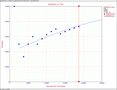
The Logistic reliability model that best fits the data is given by:

[math]\displaystyle{ R=\frac{1}{1+1.2321\cdot \ \,{{e}^{-0.0985T}}}\,\! }[/math]

The following figure shows the Reliability vs. Time plot.

Example: Logistic for Grouped per Configuration Data

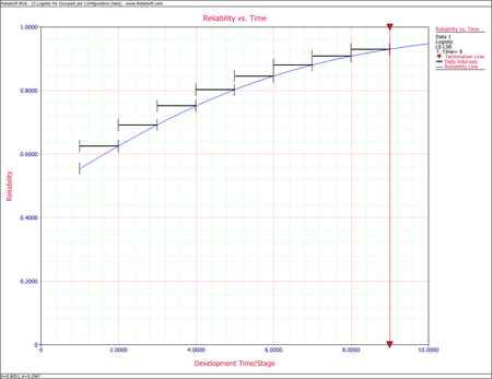
Some equipment underwent testing in different stages. The testing may have been performed in subsequent days, weeks or months with an unequal number of units tested every day. Each group was tested and several failures occurred. The data set is given in columns 1 and 2 of the following table. Find the Logistic model that best fits the data, and plot it along with the reliability observed from the raw data.

Grouped per Configuration Data

Number of Units	Number of Failures	[math]\displaystyle{ T_i\,\! }[/math]	Observed Reliability
10	5	0	0.5000
8	3	1	0.6250
9	3	2	0.6667
9	2	3	0.7778
10	2	4	0.8000
10	1	5	0.9000
10	1	6	0.9000
10	1	7	0.9000
10	1	8	0.9000

Solution

The observed reliability is [math]\displaystyle{ 1-\tfrac{\#\text{ of failures}}{\#\text{ of units}}\,\! }[/math] and the last column of the table above shows the values for each group. With [math]\displaystyle{ N=9\,\! }[/math], the least square estimator [math]\displaystyle{ \overline{Y} }[/math] becomes:

[math]\displaystyle{ \begin{align} \bar{Y}= & \frac{1}{9}\underset{i=0}{\overset{8}{\mathop \sum }}\,\ln \left( \frac{1}{{{R}_{i}}}-1 \right) \\ = & -1.4036 \end{align}\,\! }[/math]

and:

[math]\displaystyle{ \begin{align} \bar{T}= & \frac{1}{9}\underset{i=0}{\overset{8}{\mathop \sum }}\,{{T}_{i}} \\ = & 4 \\ \underset{i=0}{\overset{8}{\mathop \sum }}\,T_{i}^{2}= & 204 \\ \underset{i=0}{\overset{8}{\mathop \sum }}\,{{T}_{i}}{{Y}_{i}}= & -68.33 \end{align}\,\! }[/math]

Now from the least squares estimators, [math]\displaystyle{ \hat{b_{i}}\,\! }[/math] and [math]\displaystyle{ \hat{b_{0}}\,\! }[/math], we have:

[math]\displaystyle{ \begin{align} {{{\hat{b}}}_{1}}= & \frac{\underset{i=0}{\overset{8}{\mathop{\sum }}}\,{{T}_{i}}{{Y}_{i}}-N\cdot \bar{T}\cdot \bar{Y}}{\underset{i=0}{\overset{8}{\mathop{\sum }}}\,T_{i}^{2}-N\cdot {{{\bar{T}}}^{2}}} \\ = & \frac{-68.33-9\cdot 4\cdot \left( -1.4036 \right)}{204-9\cdot {{4}^{2}}} \\ = & -0.2967 \\ & \\ {{{\hat{b}}}_{0}}= & \bar{Y}-{{{\hat{b}}}_{1}}\bar{T} \\ = & \left( -1.4036 \right)-\left( -0.2967 \right)\cdot 4.0 \\ = & -0.2168 \end{align}\,\! }[/math]

Therefore:

[math]\displaystyle{ \begin{align} \widehat{b}= & {{e}^{-0.2168}} \\ = & 0.8051 \\ \widehat{k}= & -(-0.2967) \\ = & 0.2967 \end{align}\,\! }[/math]

The Logistic reliability model that best fits the data is given by:

[math]\displaystyle{ R=\frac{1}{1+0.8051\cdot \ \,{{e}^{-0.2967T}}}\,\! }[/math]

The figure below shows the Reliability vs. Time plot.

Confidence Bounds

Least squares is used to estimate the parameters of the following Logistic model.

[math]\displaystyle{ \ln (\frac{1}{{{{\hat{R}}}_{i}}}-1)=\ln (b)-k{{T}_{i}}\,\! }[/math]

Thus, the confidence bounds on the parameter [math]\displaystyle{ b\,\! }[/math] are given by:

[math]\displaystyle{ b=\hat{b}{{e}^{{{t}_{n-2,\alpha /2}}SE(\ln \hat{b})}}\,\! }[/math]

where:

[math]\displaystyle{ \begin{align} SE(\ln \hat{b})&=\sigma \cdot \sqrt{\frac{\underset{i=1}{\overset{n}{\mathop{\sum }}}\,{{({{T}_{i}})}^{2}}}{n\cdot {{S}_{xx}}}},\ \ \ {{S}_{xx}}=\left[ \underset{i=1}{\overset{n}{\mathop \sum }}\,{{({{T}_{i}})}^{2}} \right]-\frac{1}{n}{{\left( \underset{i=1}{\overset{n}{\mathop \sum }}\,{{T}_{i}} \right)}^{2}} \\ \\ \sigma &=\sqrt{SSE/(n-2)} \end{align}\,\! }[/math]

and the confidence bounds on the parameter [math]\displaystyle{ k\,\! }[/math] are:

[math]\displaystyle{ k=\hat{k}\pm {{t}_{n-2,\alpha /2}}SE(\hat{k})\,\! }[/math]

where:

[math]\displaystyle{ SE(\hat{k})=\frac{\sigma }{\sqrt{{{S}_{xx}}}},\ \ {{S}_{xx}}=\left[ \underset{i=1}{\overset{n}{\mathop \sum }}\,{{({{T}_{i}})}^{2}} \right]-\frac{1}{n}{{\left( \underset{i=1}{\overset{n}{\mathop \sum }}\,{{T}_{i}} \right)}^{2}}\,\! }[/math]

Since the reliability is always between 0 and 1, the logit transformation is used to obtain the confidence bounds on reliability, which is:

[math]\displaystyle{ CB=\frac{{{{\hat{R}}}_{i}}}{{{{\hat{R}}}_{i}}+(1-{{{\hat{R}}}_{i}}){{e}^{\pm {{z}_{\alpha }}{{{\hat{\sigma }}}_{R}}/\left[ {{{\hat{R}}}_{i}}(1-{{{\hat{R}}}_{i}}) \right]}}}\,\! }[/math]

Example: Logistic Confidence Bounds

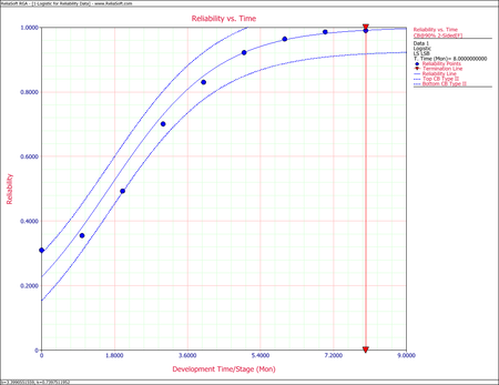
For the data given above for the reliability data example, calculate the 2-sided 90% confidence bounds under the Logistic model for the following:

1. The parameters [math]\displaystyle{ b\,\! }[/math] and [math]\displaystyle{ k\,\! }[/math].
2. Reliability at month 5.

Solution

1. The values of [math]\displaystyle{ \hat{b}\,\! }[/math] and [math]\displaystyle{ \hat{k}\,\! }[/math] that were estimated from the least squares analysis in the reliability data example are:

   [math]\displaystyle{ \begin{align} \widehat{b}= & 3.3991 \\ \widehat{\alpha }= & 0.7398 \end{align}\,\! }[/math]

   Thus, the 2-sided 90% confidence bounds on parameter [math]\displaystyle{ b\,\! }[/math] are:

   [math]\displaystyle{ \begin{align} {{b}_{lower}}= & 2.5547 \\ {{b}_{upper}}= & 4.5225 \end{align}\,\! }[/math]

   The 2-sided 90% confidence bounds on parameter [math]\displaystyle{ k\,\! }[/math] are:

   [math]\displaystyle{ \begin{align} {{k}_{lower}}= & 0.6798 \\ {{k}_{upper}}= & 0.7997 \end{align}\,\! }[/math]

2. First, calculate the reliability estimation at month 5:

   [math]\displaystyle{ \begin{align} {{R}_{5}}= & \frac{1}{1+b{{e}^{-5k}}} \\ = & 0.9224 \end{align}\,\! }[/math]

   Thus, the 2-sided 90% confidence bounds on reliability at month 5 are:

   [math]\displaystyle{ \begin{align} {{[{{R}_{5}}]}_{lower}}= & 0.8493 \\ {{[{{R}_{5}}]}_{upper}}= & 0.9955 \end{align}\,\! }[/math]

   The next figure shows a graph of the reliability plotted with 2-sided 90% confidence bounds.
   

More Examples

Auto Transmission Reliability Data

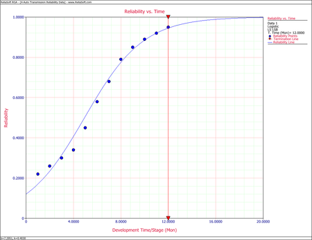
The following table presents the reliabilities observed monthly for an automobile transmission that was tested for one year.

1. Find a Logistic reliability growth curve that best represents the data.
2. Plot it comparatively with the raw data.
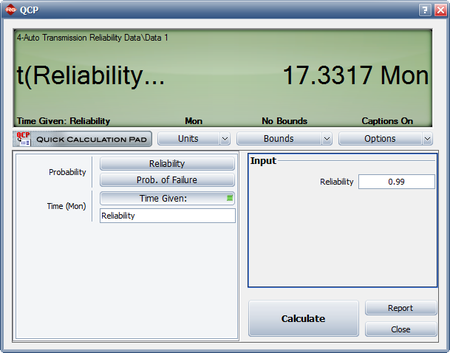
3. If design changes continue to be incorporated and the testing continues, when will the reliability goal of 99% be achieved?
4. If design changes continue to be incorporated and the testing continues, what will be the attainable reliability at the end of January the following year?

Reliability Data

Month	Observed Reliability(%)
June	22
July	26
August	30
September	34
October	45
November	58
December	68
January	79
February	85
March	89
April	92
May	95

Solution

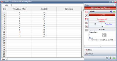
1. The next figure shows the entered data and the estimated parameters.
   
   

   
   

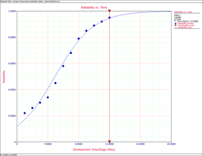
2. The next figure displays the Reliability vs. Time plot.
   
   

   
   

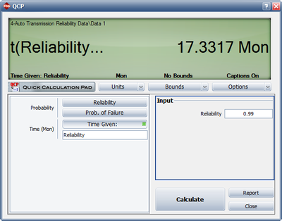
3. Using the QCP, the next figure displays, in months, when the reliability goal of 99% will be achieved.
   
   

   
   

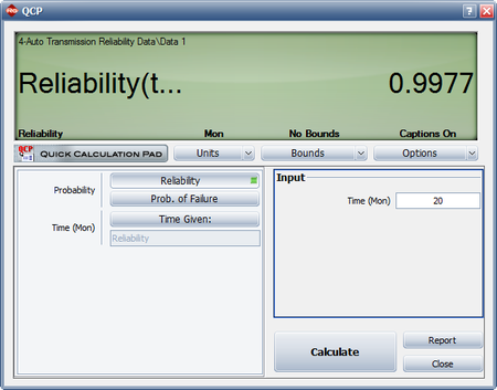
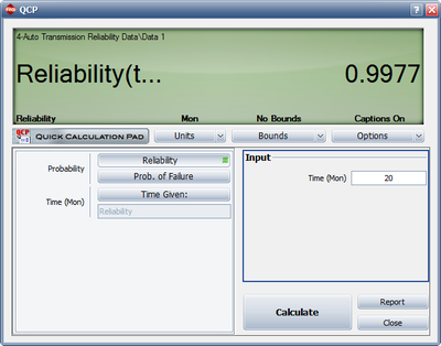
4. The last figure shows the reliability at the end of January the following year (i.e., after 20 months of testing and development).
   
   

   
   

Sequential Data from Missile Launch Test

The following table presents the results for a missile launch test. The test consisted of 20 attempts. If the missile launched, it was recorded as a success. If not, it was recorded as a failure. Note that, at this development stage, the test did not consider whether or not the target was destroyed.

1. Find a Logistic reliability growth curve that best represents the data.
2. Plot it comparatively with the raw data.
3. If design changes continue to be incorporated and the testing continues, when will the reliability goal of 99.5% with a 90% confidence level be achieved?
4. If design changes continue to be incorporated and the testing continues, what will be the attainable reliability at the end of the 35th launch?

Sequential Success/Failure Data

Launch Number	Result
1	F
2	F
3	S
4	F
5	F
6	S
7	S
8	S
9	F
10	S
11	F
12	S
13	S
14	S
15	S
16	S
17	S
18	S
19	S
20	S

Solution

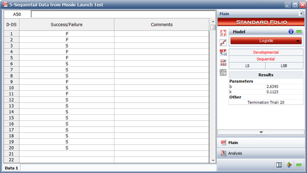
1. The next figure shows the entered data and the estimated parameters.
   
   
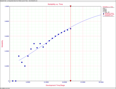
2. The next figure displays the Reliability vs. Time plot.
   
   
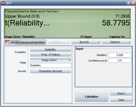
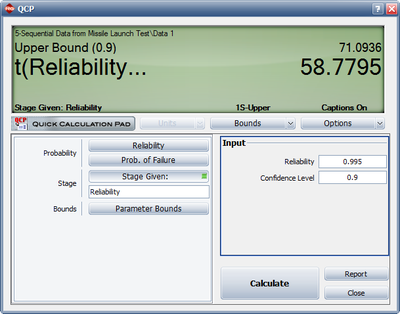
3. The next figure displays the number of launches before the reliability goal of 99.5% will be achieved with a 90% confidence level.
   
   
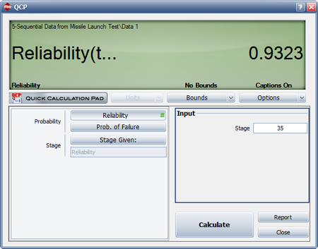
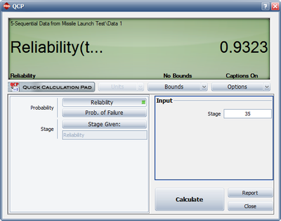
4. The next figure displays the reliability achieved after the 35th launch.
   
   

Sequential Data with Failure Modes

Consider the data given in the previous example. Now suppose that the engineers assigned failure modes to each failure and that the appropriate corrective actions were taken.

The table below presents the data.

1. Find the Logistic reliability growth curve that best represents the data.
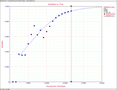
2. Plot it comparatively with the raw data.
3. If design changes continue to be incorporated and the testing continues, when will the reliability goal of 99.50% be achieved?
4. If design changes continue to be incorporated and the testing continues, what will be the attainable reliability at the end of the 35th launch?

Sequential Success/Failure Data with Modes

Launch Number	Result	Mode
1	F	2
2	F	1
3	S
4	F	3
5	F	3
6	S
7	S
8	S
9	F	2
10	S
11	F	1
12	S
13	S
14	S
15	S
16	S
17	S
18	S
19	S
20	S

Solution

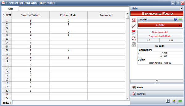
1. The next figure shows the entered data and the estimated parameters.
   
   
   
   
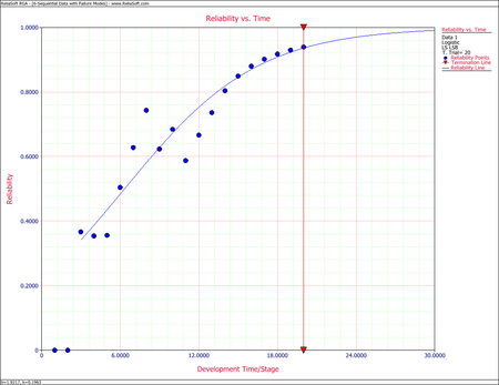
2. The next figure displays the Reliability vs. Time plot.
   
   
   
   
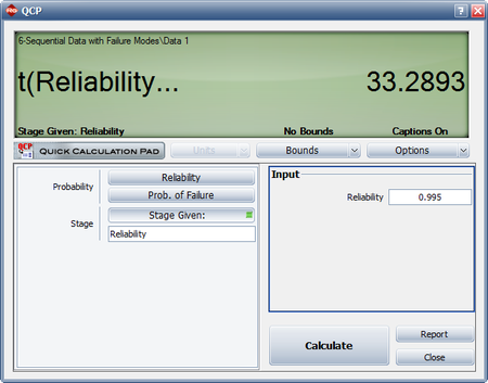
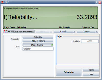
3. The next figure displays the number of launches before the reliability goal of 99.5% will be achieved.
   
   
   
   
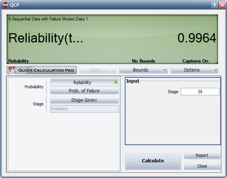
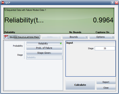
4. The last figure displays the reliability after the 35th launch.
   
   

Confidence Bounds

Least squares is used to estimate the parameters of the following Logistic model.

[math]\displaystyle{ \ln (\frac{1}{{{{\hat{R}}}_{i}}}-1)=\ln (b)-k{{T}_{i}} }[/math]

Thus the confidence bounds on the parameters are given by:

[math]\displaystyle{ b=\hat{b}{{e}^{{{t}_{n-2,\alpha /2}}SE(\ln \hat{b})}} }[/math]

where:

[math]\displaystyle{ SE(\ln \hat{b})=\sigma \cdot \sqrt{\frac{\underset{i=1}{\overset{n}{\mathop{\sum }}}\,{{({{T}_{i}})}^{2}}}{n\cdot {{S}_{xx}}}},\ \ \ {{S}_{xx}}=\left[ \underset{i=1}{\overset{n}{\mathop \sum }}\,{{({{T}_{i}})}^{2}} \right]-\frac{1}{n}{{\left( \underset{i=1}{\overset{n}{\mathop \sum }}\,{{T}_{i}} \right)}^{2}} }[/math]

[math]\displaystyle{ \sigma =\sqrt{SSE/(n-2)} }[/math]

and:

[math]\displaystyle{ k=\hat{k}\pm {{t}_{n-2,\alpha /2}}SE(\hat{k}) }[/math]

where:

[math]\displaystyle{ SE(\hat{k})=\frac{\sigma }{\sqrt{{{S}_{xx}}}},\ \ {{S}_{xx}}=\left[ \underset{i=1}{\overset{n}{\mathop \sum }}\,{{({{T}_{i}})}^{2}} \right]-\frac{1}{n}{{\left( \underset{i=1}{\overset{n}{\mathop \sum }}\,{{T}_{i}} \right)}^{2}} }[/math]

Since the reliability is always between 0 and 1, the logit transformation is used to obtain the confidence bounds on reliability.

[math]\displaystyle{ CB=\frac{{{{\hat{R}}}_{i}}}{{{{\hat{R}}}_{i}}+(1-{{{\hat{R}}}_{i}}){{e}^{\pm {{z}_{\alpha }}{{{\hat{\sigma }}}_{R}}/\left[ {{{\hat{R}}}_{i}}(1-{{{\hat{R}}}_{i}}) \right]}}} }[/math]

Example 4
For the data given for Example 1 in Table 8.1, calculate the 2-sided 90% confidence bounds under the Logistic model for the following:

1) The parameters [math]\displaystyle{ b }[/math] and [math]\displaystyle{ k }[/math] .

2) Reliability at month 5.

Solution

1) The values of [math]\displaystyle{ \widehat{b} }[/math] and [math]\displaystyle{ \widehat{k} }[/math] estimated from the least squares analysis in Example 1:

[math]\displaystyle{ \begin{align} & \widehat{b}= & 3.3991 \\ & \widehat{\alpha }= & 0.7398 \end{align} }[/math]

Thus the 2-sided 90% confidence bounds on parameter [math]\displaystyle{ b }[/math] using Eqn. (LogCBb) are:

[math]\displaystyle{ \begin{align} & {{b}_{lower}}= & 2.5547 \\ & {{b}_{upper}}= & 4.5225 \end{align} }[/math]

The 2-sided 90% confidence bounds on parameter [math]\displaystyle{ k }[/math] using Eqn. (logCBk) are:

[math]\displaystyle{ \begin{align} & {{k}_{lower}}= & 0.6798 \\ & {{k}_{upper}}= & 0.7997 \end{align} }[/math]

2) First calculate the reliability estimation at month 5:

[math]\displaystyle{ \begin{align} & {{R}_{5}}= & \frac{1}{1+b{{e}^{-5k}}} \\ & = & 0.9224 \end{align} }[/math]

Thus the 2-sided 90% confidence bounds on reliability at month 5 using Eqn. (LogCR) are:

[math]\displaystyle{ \begin{align} & {{[{{R}_{5}}]}_{lower}}= & 0.8493 \\ & {{[{{R}_{5}}]}_{upper}}= & 0.9955 \end{align} }[/math]

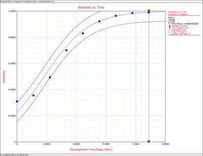
Figure Logig86 shows a graph of the reliability plotted with 2-sided 90% confidence bounds.

Logistic Reliability vs. Time plot with 2-sided 90% confidence bounds.

General Examples

Example 5

Table 8.4 presents the reliabilities observed monthly for an automobile transmission that was tested for one year.

1) Find a Logistic reliability growth curve that best represents the data.

2) Plot it comparatively with the raw data.

3) If design changes continue to be incorporated and the testing continues, when will the reliability goal of 99% be achieved?

4) If design changes continue to be incorporated and the testing continues, what will be the attainable reliability at the end of January the following year?

Table 8.4 - Reliability data

Month	Observed Reliability(%)
June	22
July	26
August	30
September	34
October	45
November	58
December	68
January	79
February	85
March	89
April	92
May	95

Entered data and the estimated Logistic parameters.

Reliability vs. Time plot.

When the reliability goal of 99% will be achieved.

The reliability at the end of the following January (month=20)

Solution to Example 5

1) Figure Loge21 shows the estimated parameters.

2) Figure Loge22 displays the Reliability vs. Time plot.

3) Using the QCP, Figure Loge23 displays when the reliability goal of 99% will be achieved.

4) Figure Loge24 shows the reliability at the end of January the following year (i.e. after 20 months of testing and development).

Example 6

Table 8.5 presents the results for a missile launch test. The test consisted of 20 attempts. If the missile launched, it was recorded as a success. If not, it was recorded as a failure. Note that, at this development stage, the test did not consider whether or not the target was destroyed.

1) Find a Logistic reliability growth curve that best represents the data.

2) Plot it comparatively with the raw data.

3) If design changes continue to be incorporated and the testing continues, when will the reliability goal of 99.5% with a 90% confidence level be achieved?

4) If design changes continue to be incorporated and the testing continues, what will be the attainable reliability at the end of the 35th launch?

Table 8.5 - Sequential success/failure data

Launch Number	Result
1	F
2	F
3	S
4	F
5	F
6	S
7	S
8	S
9	F
10	S
11	F
12	S
13	S
14	S
15	S
16	S
17	S
18	S
19	S
20	S

Solution to Example 6

1) Figure Loge31 shows the entered data and the estimated parameters.

2) Figure Loge32 displays the Reliability vs. Time plot.

3) Figure Loge33 displays when the reliability goal of 99.5% will be achieved with a 90% confidence level.

4) Figure Loge34 displays the reliability achieved after the 35th launch.

Entered data and the estimated logistic parameters.

Reliability vs. Time plot.

When the reliability goal of 99.5% with a 90% confidence level will be achieved.

The reliability at the end of the 35th launch.

Example 7

Consider the data given for the missile launch test in Example 6. Now suppose that the engineers assigned failure modes to each failure and that the appropriate corrective actions were taken.
Table 8.6 presents the data.

1) Find the Logistic reliability growth curve that best represents the data.

2) Plot it comparatively with the raw data.

3) If design changes continue to be incorporated and the testing continues, when will the reliability goal of 99.50% be achieved?

4) If design changes continue to be incorporated and the testing continues, what will be the attainable reliability at the end of the 35th launch?

Table 8.6 - Sequential success/failure data with modes

Launch Number	Result	Mode
1	F	2
2	F	1
3	S
4	F	3
5	F	3
6	S
7	S
8	S
9	F	2
10	S
11	F	1
12	S
13	S
14	S
15	S
16	S
17	S
18	S
19	S
20	S

Solution to Example 7

1) Figure Loge51 shows the estimated parameters.

2) Figure Loge52 displays the Reliability vs. Time plot.

3) Figure Loge53 displays when the reliability goal of 99.5% will be achieved.

4) Figure Loge54 displays the reliability after the 35th launch.

Entered data and the estimated Logistic parameters.

Reliability vs. Time plot.

Calculate when the reliability goal of 99.5% will be achieved.

Calculate the reliability at the end of the 35th launch.