The Mixed Weibull Distribution: Difference between revisions
| Line 16: | Line 16: | ||
{{background of weibull distribution}} | {{background of weibull distribution}} | ||
{{mixed weibull parameter estimation}} | |||
{{mixed weibull | |||
===Using the Mixed Weibull Distribution in Weibull++=== | ===Using the Mixed Weibull Distribution in Weibull++=== | ||
Revision as of 18:43, 4 January 2012
Other Distributions
Besides the Weibull, exponential, normal and lognormal, there are other distributions that are used to model reliability and life data. However, these four represent the most prominent distributions in Weibull++. In this chapter, we will discuss other distributions that are used under special circumstances: the mixed Weibull, the generalized gamma, the Gumbel, the logistic and the loglogistic distributions.
Mixed Weibull Distribution
The mixed Weibull distribution (also known as a multimodal Weibull) is used to model data that do not fall on a straight line on a Weibull probability plot. Data of this type, particularly if the data points follow an S-shape on the probability plot, may be indicative of more than one failure mode at work in the population of failure times. Field data from a given mixed population may frequently represent multiple failure modes. The necessity of determining the life regions where these failure modes occur is apparent when it is realized that the times-to-failure for each mode may follow a distinct Weibull distribution, thus requiring individual mathematical treatment. Another reason is that each failure mode may require a different design change to improve the component's reliability [19].
A decreasing failure rate is usually encountered during the early life period of components when the substandard components fail and are removed from the population. The failure rate continues to decrease until all such substandard components fail and are removed. This corresponds to a decreasing failure rate. The Weibull distribution having [math]\displaystyle{ \beta \lt 1 }[/math] is often used to depict this life characteristic.
A second type of failure prevails when the components fail by chance alone and their failure rate is nearly constant. This can be caused by sudden, unpredictable stress applications that have a stress level above those to which the product is designed. Such failures tend to occur throughout the life of a component. The distributions most often used to describe this failure rate characteristic are the exponential distribution and the Weibull distribution with [math]\displaystyle{ \beta \approx 1 }[/math] .
A third type of failure is characterized by a failure rate that increases as operating hours are accumulated. Usually, wear has started to set in and this brings the component's performance out of specification. As age increases further, this wear-out process removes more and more components until all components fail. The normal distribution and the Weibull distribution with a [math]\displaystyle{ \beta \gt 1 }[/math] have been successfully used to model the times-to-failure distribution during the wear-out period.
Several different failure modes may occur during the various life periods. A methodology is needed to identify these failure modes and determine their failure distributions and reliabilities. This section presents a procedure whereby the proportion of units failing in each mode is determined and their contribution to the reliability of the component is quantified. From this reliability expression, the remaining major reliability functions, the probability density, the failure rate and the conditional-reliability functions are calculated to complete the reliability analysis of such mixed populations.
Template loop detected: Template:Background of weibull distribution
Template loop detected: Template:Mixed weibull parameter estimation
Using the Mixed Weibull Distribution in Weibull++
To use the mixed Weibull distribution, simply select the Mixed option under Parameters/Type, and click the Calculate icon. A window will appear asking you which form of the mixed Weibull you would like to use, i.e. S = 2, 3 or 4. In other words, How many subpopulations would you like to consider?
Simply select the number of subpopulations you would like to consider and click OK. The application will automatically calculate the parameters of each subpopulation for you.
Viewing the Calculated Parameters
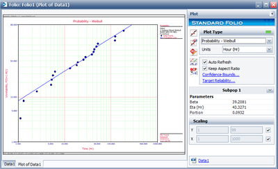
When using the Mixed Weibull option, the parameters given in the result area apply to different subpopulations. To view the results for a particular subpopulation, select the subpopulation, as shown next.
About the Calculated Parameters
Weibull++ uses the numbers 1, 2, 3 and 4 (or first, second, third and fourth subpopulation) to identify each subpopulation. These are just designations for each subpopulation, and they are ordered based on the value of the scale parameter, [math]\displaystyle{ \eta }[/math] . Since the equation used is additive or:
- [math]\displaystyle{ {{R}_{1,..,S}}(T)=\underset{i=1}{\overset{S}{\mathop \sum }}\,\frac{{{N}_{i}}}{N}{{e}^{-{{\left( \tfrac{T}{{{\eta }_{i}}} \right)}^{{{\beta }_{i}}}}}} }[/math]
the order of the subpopulations which are given the designation 1, 2, 3, or 4 is of no consequence. For consistency, the application will always return the order of the results based on the magnitude of the scale parameter.
Mixed Weibull, Other Uses
Reliability Bathtub Curves
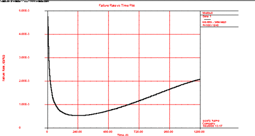
A reliability bathtub curve is nothing more than the graph of the failure rate versus time, over the life of the product. In general, the life stages of the product consist of early, chance and wear-out. Weibull++ allows you to plot this by simply selecting the failure rate plot, as shown next.
Determination of the Burn-in Period
If the failure rate goal is known, then the burn-in period can be found from the failure rate plot by drawing a horizontal line at the failure rate goal level and then finding the intersection with the failure rate curve. Next, drop vertically at the intersection, and read off the burn-in time from the time axis. This burn-in time helps insure that the population will have a failure rate that is at least equal to or lower than the goal after the burn-in period. The same could also be obtained using the Function Wizard and generating different failure rates based on time increments. Using these generated times and the corresponding failure rates, one can decide on the optimum burn-in time versus the corresponding desired failure rate.
A Mixed Weibull Example
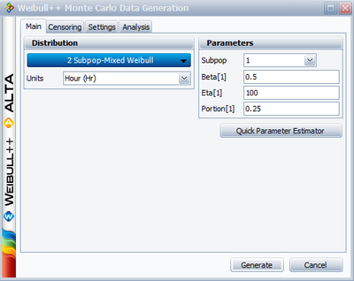
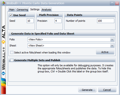
We will illustrate mixed Weibull analysis using a Monte Carlo generated set of data. To repeat this example, generate data from a two-parameter Weibull distribution, using the Weibull++ Monte Carlo data window. The following figures illustrate the required steps, inputs and results.
• In the Monte Carlo window, enter the values and select the options shown below for subpopulation 1.
Switch to subpopulation 2 and make the selection shown below. Click Generate.
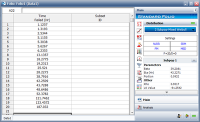
• After the data has been generated, choose the Weibull distribution and select Mixed for the Parameters/Type. Click the Calculate icon
The results for subpopulation 1 are shown next. (Note that your results could be different due to the randomness of the simulation.)
The results for subpopulation 2 are shown next (Note that your results could be different due to the randomness of the simulation.)
The Weibull probability plot for this data is shown next (Note that your results could be different due to the randomness of the simulation.)


