The Normal Distribution: Difference between revisions
| Line 16: | Line 16: | ||
{{normal distribution estimation of the parameters}} | {{normal distribution estimation of the parameters}} | ||
{{normal distribution confidence bounds}} | |||
==Bayesian Confidence Bounds== | ==Bayesian Confidence Bounds== | ||
Revision as of 17:45, 4 January 2012
The Normal Distribution
The normal distribution, also known as the Gaussian distribution, is the most widely-used general purpose distribution. It is for this reason that it is included among the lifetime distributions commonly used for reliability and life data analysis. There are some who argue that the normal distribution is inappropriate for modeling lifetime data because the left-hand limit of the distribution extends to negative infinity. This could conceivably result in modeling negative times-to-failure. However, provided that the distribution in question has a relatively high mean and a relatively small standard deviation, the issue of negative failure times should not present itself as a problem. Nevertheless, the normal distribution has been shown to be useful for modeling the lifetimes of consumable items, such as printer toner cartridges.
Template loop detected: Template:Normal probability density function
Template loop detected: Template:Normal statistical properties
Template loop detected: Template:Characteristics of the normal distribution
Template loop detected: Template:Normal distribution estimation of the parameters
Template loop detected: Template:Normal distribution confidence bounds
Bayesian Confidence Bounds
Bounds on Parameters
From Chapter 5, we know that the marginal posterior distribution of [math]\displaystyle{ \mu }[/math] can be written as:
- [math]\displaystyle{ \begin{align} f(\mu |Data)= & \int_{0}^{\infty }f(\mu ,\sigma |Data)d\sigma \\ = & \frac{\int_{0}^{\infty }L(Data|\mu ,\sigma )\varphi (\mu )\varphi (\sigma )d\sigma }{\int_{0}^{\infty }\int_{-\infty }^{\infty }L(Data|\mu ,\sigma )\varphi (\mu )\varphi (\sigma )d\mu d\sigma } \end{align} }[/math]
- where:
[math]\displaystyle{ \varphi (\sigma ) }[/math] = [math]\displaystyle{ \tfrac{1}{\sigma } }[/math] is the non-informative prior of [math]\displaystyle{ \sigma }[/math] .
- [math]\displaystyle{ \varphi (\mu ) }[/math] is a uniform distribution from - [math]\displaystyle{ \infty }[/math] to + [math]\displaystyle{ \infty }[/math] , the non-informative prior of [math]\displaystyle{ \mu . }[/math]
Using the above prior distributions, [math]\displaystyle{ f(\mu |Data) }[/math] can be rewritten as:
- [math]\displaystyle{ f(\mu |Data)=\frac{\int_{0}^{\infty }L(Data|\mu ,\sigma )\tfrac{1}{\sigma }d\sigma }{\int_{0}^{\infty }\int_{-\infty }^{\infty }L(Data|\mu ,\sigma )\tfrac{1}{\sigma }d\mu d\sigma } }[/math]
The one-sided upper bound of [math]\displaystyle{ \mu }[/math] is:
- [math]\displaystyle{ CL=P(\mu \le {{\mu }_{U}})=\int_{-\infty }^{{{\mu }_{U}}}f(\mu |Data)d\mu }[/math]
The one-sided lower bound of [math]\displaystyle{ \mu }[/math] is:
- [math]\displaystyle{ 1-CL=P(\mu \le {{\mu }_{L}})=\int_{-\infty }^{{{\mu }_{L}}}f(\mu |Data)d\mu }[/math]
The two-sided bounds of [math]\displaystyle{ \mu }[/math] are:
- [math]\displaystyle{ CL=P({{\mu }_{L}}\le \mu \le {{\mu }_{U}})=\int_{{{\mu }_{L}}}^{{{\mu }_{U}}}f(\mu |Data)d\mu }[/math]
The same method can be used to obtained the bounds of [math]\displaystyle{ \sigma }[/math].
Bounds on Time (Type 1)
The reliable life for the normal distribution is:
- [math]\displaystyle{ T=\mu +\sigma {{\Phi }^{-1}}(1-R) }[/math]
The one-sided upper bound on time is:
- [math]\displaystyle{ CL=\underset{}{\overset{}{\mathop{\Pr }}}\,(T\le {{T}_{U}})=\underset{}{\overset{}{\mathop{\Pr }}}\,(\mu +\sigma {{\Phi }^{-1}}(1-R)\le {{T}_{U}}) }[/math]
Eqn. (1SCBT) can be rewritten in terms of [math]\displaystyle{ \mu }[/math] as:
- [math]\displaystyle{ CL=\underset{}{\overset{}{\mathop{\Pr }}}\,(\mu \le {{T}_{U}}-\sigma {{\Phi }^{-1}}(1-R)) }[/math]
From the posterior distribution of [math]\displaystyle{ \mu \ \ : }[/math]
- [math]\displaystyle{ CL=\frac{\int_{0}^{\infty }\int_{-\infty }^{{{T}_{U}}-\sigma {{\Phi }^{-1}}(1-R)}L(\sigma ,\mu )\tfrac{1}{\sigma }d\mu d\sigma }{\int_{0}^{\infty }\int_{-\infty }^{\infty }L(\sigma ,\mu )\tfrac{1}{\sigma }d\mu d\sigma } }[/math]
The same method can be applied for one-sided lower bounds and two-sided bounds on time.
Bounds on Reliability (Type 2)
The one-sided upper bound on reliability is:
- [math]\displaystyle{ CL=\underset{}{\overset{}{\mathop{\Pr }}}\,(R\le {{R}_{U}})=\underset{}{\overset{}{\mathop{\Pr }}}\,(\mu \le T-\sigma {{\Phi }^{-1}}(1-{{R}_{U}})) }[/math]
From the posterior distribution of [math]\displaystyle{ \mu \ \ : }[/math]
- [math]\displaystyle{ CL=\frac{\int_{0}^{\infty }\int_{-\infty }^{T-\sigma {{\Phi }^{-1}}(1-{{R}_{U}})}L(\sigma ,\mu )\tfrac{1}{\sigma }d\mu d\sigma }{\int_{0}^{\infty }\int_{-\infty }^{\infty }L(\sigma ,\mu )\tfrac{1}{\sigma }d\mu d\sigma } }[/math]
The same method can be used to calculate the one-sided lower bounds and the two-sided bounds on reliability.
General Examples
Example 8
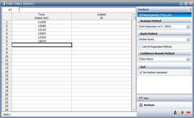
Six units are tested to failure with the following hours-to-failure data obtained: 12125, 11260, 12080, 12825, 13550 and 14670 hours. Assuming the data are normally distributed, do the following: 8-1. Find the parameters for the data. (Use Rank Regression on X to duplicate the results shown in this example.) 8-2. Obtain the probability plot for the data with 90%, two-sided Type 1 confidence bounds. 8-3. Obtain the [math]\displaystyle{ pdf }[/math] plot for these data.
Solutions to Example 8
8-1. The next figure shows the data as entered in Weibull++, as well as the calculated parameters.
[math]\displaystyle{ }[/math]
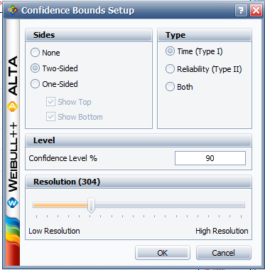
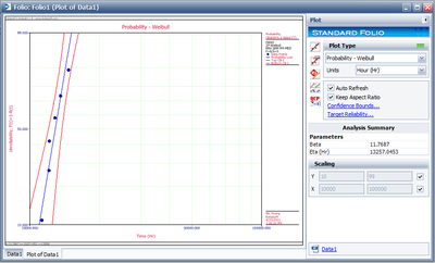
8-2. Obtain the probability plot as before. To plot confidence bounds, from the Plot Options menu choose Confidence Bounds and then Show Confidence Bounds. On the Type and Settings page of the Confidence Bounds window, select Two Sided Bounds, make sure Type 1 is selected, and then enter 90 in the Confidence level, % box, and click OK, as shown next.
[math]\displaystyle{ }[/math]
The following plot should appear on your screen:
[math]\displaystyle{ }[/math]
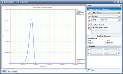
8-3. From the Special Plot Type menu choose Pdf Plot. The following plot should appear on your screen.
[math]\displaystyle{ }[/math]
Example 9
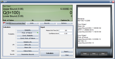
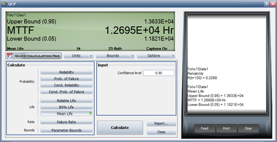
Using the data and results from the previous example (and RRX), do the following: 9-1. Using the Quick Calculation Pad, determine the reliability for a mission of 11,000 hours, as well as the upper and lower two-sided 90% confidence limit on this reliability. 9-2. Using the Quick Calculation Pad, determine the MTTF, as well as the upper and lower two-sided 90% confidence limit on this MTTF.
Solutions to Example 9
Both of these results are easily obtained from the QCP. The QCP with results for both cases is shown in the next two figures.
Example 10
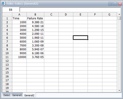
Using the data from Example 8, and using the rank regression on X analysis method (RRX), obtain tabulated values for the failure rate for 10 different mission end times. The mission end times are 1,000 to 10,000 hours, using increments of 1,000 hours.
Solution to Example 10
This can be easily accomplished via the use of the Function Wizard, available in either Weibull++'s Reports or the General Spreadsheet. (For more information on these features, please refer to the Weibull++ User's Guide.) We will illustrate this using the General Spreadsheet.
First, click on Insert General Spread Sheet from the Folio menu.
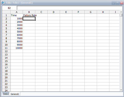
Type Time in cell A1 and Failure Rate in cell B1. Then enter 1000 through 10000 in cells A2 to A11. Finally, place the cursor into cell B2, as shown next.
Open the Function Wizard by selecting Function Wizard from the Data menu or by clicking the Function Wizard icon.
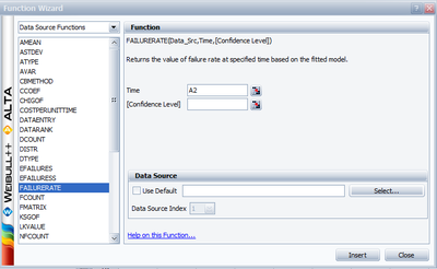
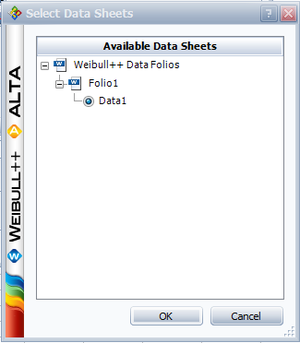
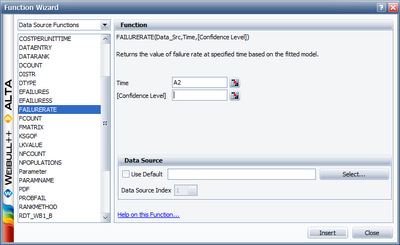
Select FAILURERATE from the list of functions. Enter A2 for Time; this indicates that the time input for the equation will be obtained from the specified cell in the worksheet. To specify the existing Weibull++ analysis that the function result will be based on, click Select... to open the Select Folio/Data Sheet window and then navigate to the desired sheet.
Click OK to close the window and return to the Function Wizard. Click Add to Equation to update the box at the bottom of the window with the function code that will be inserted into the spreadsheet.
Click Insert to close the window and insert the function code into the active cell in the General Spreadsheet. Copy the function into cells B3 through B11. One way to do this is to position the mouse over the bottom right corner of cell B2 and when the cursor turns into a plus symbol (+), click and drag the mouse to cell B11. By selecting one of the cells that you copied the function into, you can see that the cell reference was updated to match the current row, as shown next with cell B11 selected. The results are as follows:
Example 11
Eight units are being reliability tested and the following is a table of their times-to-failure:
| Table 8.3 - Non-Grouped Data Times-to-Failure with intervals (lnterval and left censored) | ||
| Data point index | Last Inspected | State End Time |
|---|---|---|
| 1 | 30 | 32 |
| 2 | 32 | 35 |
| 3 | 35 | 37 |
| 4 | 37 | 40 |
| 5 | 42 | 42 |
| 6 | 45 | 45 |
| 7 | 50 | 50 |
| 8 | 55 | 55 |
Solution to Example 11
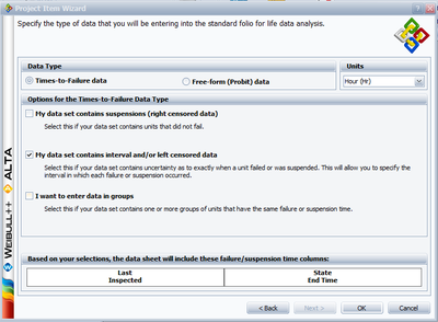
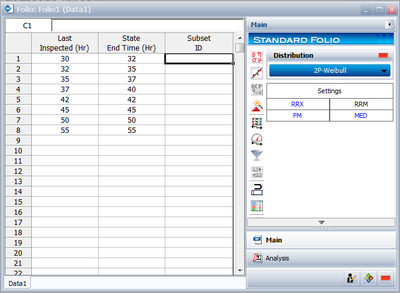
This is a sequence of interval times-to-failure. This data set can be entered into Weibull++ by creating a data sheet that can be used to analyze times-to-failure data with interval and left censored data.
[math]\displaystyle{ }[/math]
The computed parameters for maximum likelihood are:
- [math]\displaystyle{ \begin{align} & \widehat{\mu }= & 41.40 \\ & {{{\hat{\sigma }}}_{T}}= & 7.740. \end{align} }[/math]
For rank regression on x:
- [math]\displaystyle{ \begin{align} & \widehat{\mu }= & 41.40 \\ & {{{\hat{\sigma }}}_{T}}= & 9.03. \end{align} }[/math]
For rank regression on y:
- [math]\displaystyle{ \begin{align} & \widehat{\mu }= & 41.39 \\ & {{{\hat{\sigma }}}_{T}}= & 9.25. \end{align} }[/math]
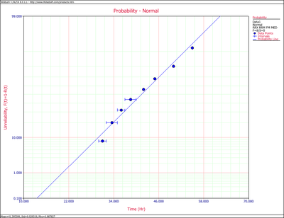
A plot of the MLE solution is shown next.
[math]\displaystyle{ }[/math]
Example 12
Eight units are being reliability tested and the following is a table of their times-to-failure:
| Table 8.4 - Non-Grouped Data ,for Example 12 | ||
| Data point index | State F or S | State End Time |
|---|---|---|
| 1 | F | 2 |
| 2 | F | 5 |
| 3 | F | 11 |
| 4 | F | 23 |
| 5 | F | 29 |
| 6 | F | 37 |
| 7 | F | 43 |
| 8 | F | 59 |
Solution to Example 12
This data set can be entered into Weibull++ by creating a Data Sheet appropriate for the entry of non-grouped times-to-failure data. The computed parameters for maximum likelihood are:
- [math]\displaystyle{ \begin{align} & \widehat{\mu }= & 26.13 \\ & {{{\hat{\sigma }}}_{T}}= & 18.57 \end{align} }[/math]
For rank regression on x:
- [math]\displaystyle{ \begin{align} & \widehat{\mu }= & 26.13 \\ & {{{\hat{\sigma }}}_{T}}= & 21.64 \end{align} }[/math]
For rank regression on y:
- [math]\displaystyle{ \begin{align} & \widehat{\mu }= & 26.13 \\ & {{{\hat{\sigma }}}_{T}}= & 22.28. \end{align} }[/math]
Example 13
Nineteen units are being reliability tested and the following is a table of their times-to-failure and suspensions.
| Table 8.5 - Non-Grouped Data Times-to-Failure with Suspensions (Right Censored) | ||
| Data point index | Last Inspected | State End Time |
|---|---|---|
| 1 | F | 2 |
| 2 | S | 3 |
| 3 | F | 5 |
| 4 | S | 7 |
| 5 | F | 11 |
| 6 | S | 13 |
| 7 | S | 17 |
| 8 | S | 19 |
| 9 | F | 23 |
| 10 | F | 29 |
| 11 | S | 31 |
| 12 | F | 37 |
| 13 | S | 41 |
| 14 | F | 43 |
| 15 | S | 47 |
| 16 | S | 53 |
| 17 | F | 59 |
| 18 | S | 61 |
| 19 | S | 67 |
Solution to Example 13
This augments the previous example by adding eleven suspensions to the data set. This data set can be entered into Weibull++ by selecting the data sheet for Times to Failure and with Right Censored Data (Suspensions). The parameters using maximum likelihood are:
- [math]\displaystyle{ \begin{align} & \widehat{\mu }= & 48.07 \\ & {{{\hat{\sigma }}}_{T}}= & 28.41. \end{align} }[/math]
For rank regression on x:
- [math]\displaystyle{ \begin{align} & \widehat{\mu }= & 46.40 \\ & {{{\hat{\sigma }}}_{T}}= & 28.64. \end{align} }[/math]
For rank regression on y:
- [math]\displaystyle{ \begin{align} & \widehat{\mu }= & 47.34 \\ & {{{\hat{\sigma }}}_{T}}= & 29.96. \end{align} }[/math]
Example 14
Suppose our data set includes left and right censored, interval censored and complete data as shown in the following table.
Solution to Example 14
This data set can be entered into Weibull++ by selecting the data type Times to Failure, with Right Censored Data (Suspensions), with Interval and Left Censored Data and with Grouped Observations.
The computed parameters using maximum likelihood are:
- [math]\displaystyle{ \begin{align} & \widehat{\mu }= & 48.11 \\ & {{{\hat{\sigma }}}_{T}}= & 26.42. \end{align} }[/math]
For rank regression on x:
- [math]\displaystyle{ \begin{align} & \widehat{\mu }= & 49.99 \\ & {{{\hat{\sigma }}}_{T}}= & 30.17. \end{align} }[/math]
For rank regression on y:
- [math]\displaystyle{ \begin{align} & \widehat{\mu }= & 51.61 \\ & {{{\hat{\sigma }}}_{T}}= & 33.07. \end{align} }[/math]

