Non-Parametric Life Data Analysis
Non-parametric analysis allows the user to analyze data without assuming an underlying distribution. This can have certain advantages as well as disadvantages. The ability to analyze data without assuming an underlying life distribution avoids the potentially large errors brought about by making incorrect assumptions about the distribution. On the other hand, the confidence bounds associated with non-parametric analysis are usually much wider than those calculated via parametric analysis, and predictions outside the range of the observations are not possible. Some practitioners recommend that any set of life data should first be subjected to a non-parametric analysis before moving on to the assumption of an underlying distribution.
There are several methods for conducting a non-parametric analysis. In Weibull++, this includes the Kaplan-Meier, actuarial-simple and actuarial-standard methods. A method for attaching confidence bounds to the results of these non-parametric analysis techniques can also be developed. The basis of non-parametric life data analysis is the empirical cdf function, which is given by:
- [math]\displaystyle{ \widehat{F}(t)=\frac{observations\le t}{n}\,\! }[/math]
Note that this is similar to the Benard's approximation of the median ranks, as discussed in the Parameter Estimation chapter. The following non-parametric analysis methods are essentially variations of this concept.
Kaplan-Meier Estimator
The Kaplan-Meier estimator, also known as the product limit estimator, can be used to calculate values for non-parametric reliability for data sets with multiple failures and suspensions. The equation of the estimator is given by:
- [math]\displaystyle{ \widehat{R}({{t}_{i}})=\underset{j=1}{\overset{i}{\mathop \prod }}\,\frac{{{n}_{j}}-{{r}_{j}}}{{{n}_{j}}},\text{ }i=1,...,m\,\! }[/math]
where:
- [math]\displaystyle{ \begin{align} & m= \text{the total number of data points} \\ & n= \text{the total number of units} \end{align}\,\! }[/math]
The variable [math]\displaystyle{ {{n}_{i}}\,\! }[/math] is defined by:
- [math]\displaystyle{ {{n}_{i}}=n-\underset{j=0}{\overset{i-1}{\mathop \sum }}\,{{s}_{j}}-\underset{j=0}{\overset{i-1}{\mathop \sum }}\,{{r}_{j,}}\text{ }i=1,...,m\,\! }[/math]
where:
- [math]\displaystyle{ \begin{align} & {{r}_{j}}= \text{the number of failures in the }{{j}^{th}}\text{ data group} \\ & {{s}_{j}}= \text{the number of suspensions in the }{{j}^{th}}\text{ data group} \end{align}\,\! }[/math]
Note that the reliability estimate is only calculated for times at which one or more failures occurred. For the sake of calculating the value of [math]\displaystyle{ {{n}_{j}}\,\! }[/math] at time values that have failures and suspensions, it is assumed that the suspensions occur slightly after the failures, so that the suspended units are considered to be operating and included in the count of [math]\displaystyle{ {{n}_{j}}\,\! }[/math].
Kaplan-Meier Example
A group of 20 units are put on a life test with the following results.
Use the Kaplan-Meier estimator to determine the reliability estimates for each failure time.
Solution
Using the data and the reliability equation of the Kaplan-Meier estimator, the following table can be constructed:
As can be determined from the preceding table, the reliability estimates for the failure times are:
Actuarial-Simple Method
The actuarial-simple method is an easy-to-use form of non-parametric data analysis that can be used for multiple censored data that are arranged in intervals. This method is based on calculating the number of failures in a time interval, [math]\displaystyle{ {{r}_{j}}\,\! }[/math] versus the number of operating units in that time period, [math]\displaystyle{ {{n}_{j}}\,\! }[/math]. The equation for the reliability estimator for the standard actuarial method is given by:
- [math]\displaystyle{ \widehat{R}({{t}_{i}})=\underset{j=1}{\overset{i}{\mathop \prod }}\,\left( 1-\frac{{{r}_{j}}}{{{n}_{j}}} \right),\text{ }i=1,...,m\,\! }[/math]
where:
- [math]\displaystyle{ \begin{align} & m= \text{the total number of intervals} \\ & n= \text{the total number of units} \end{align}\,\! }[/math]
The variable [math]\displaystyle{ {{n}_{i}}\,\! }[/math] is defined by:
- [math]\displaystyle{ {{n}_{i}}=n-\underset{j=0}{\overset{i-1}{\mathop \sum }}\,{{s}_{j}}-\underset{j=0}{\overset{i-1}{\mathop \sum }}\,{{r}_{j,}}\text{ }i=1,...,m\,\! }[/math]
where:
- [math]\displaystyle{ \begin{align} & {{r}_{j}}= \text{the number of failures in interval }j \\ & {{s}_{j}}= \text{the number of suspensions in interval }j \end{align}\,\! }[/math]
Actuarial-Simple Example
A group of 55 units are put on a life test during which the units are evaluated every 50 hours. The results are:
Solution
The reliability estimates can be obtained by expanding the data table to include the calculations used in the actuarial-simple method:
As can be determined from the preceding table, the reliability estimates for the failure times are:
Actuarial-Standard Method
The actuarial-standard model is a variation of the actuarial-simple model. In the actuarial-simple method, the suspensions in a time period or interval are assumed to occur at the end of that interval, after the failures have occurred. The actuarial-standard model assumes that the suspensions occur in the middle of the interval, which has the effect of reducing the number of available units in the interval by half of the suspensions in that interval or:
- [math]\displaystyle{ n_{i}^{\prime }={{n}_{i}}-\frac{{{s}_{i}}}{2}\,\! }[/math]
With this adjustment, the calculations are carried out just as they were for the actuarial-simple model or:
- [math]\displaystyle{ \widehat{R}({{t}_{i}})=\underset{j=1}{\overset{i}{\mathop \prod }}\,\left( 1-\frac{{{r}_{j}}}{n_{j}^{\prime }} \right),\text{ }i=1,...,m\,\! }[/math]
Actuarial-Standard Example
Use the data set from the Actuarial-Simple example and analyze it using the actuarial-standard method.
Solution
The solution to this example is similar to that in the Actuarial-Simple example, with the exception of the inclusion of the [math]\displaystyle{ n_{i}^{\prime }\,\! }[/math] term, which is used in the equation for the actuarial-standard method. Applying this equation to the data, we can generate the following table:
As can be determined from the preceding table, the reliability estimates for the failure times are:
Non-Parametric Confidence Bounds
Confidence bounds for non-parametric reliability estimates can be calculated using a method similar to that of parametric confidence bounds. The difficulty in dealing with nonparametric data lies in the estimation of the variance. To estimate the variance for non-parametric data, Weibull++ uses Greenwood's formula [27]:
- [math]\displaystyle{ \widehat{Var}(\hat{R}({{t}_{i}}))={{\left[ \hat{R}({{t}_{i}}) \right]}^{2}}\cdot \underset{j=1}{\overset{i}{\mathop \sum }}\,\frac{\tfrac{{{r}_{j}}}{{{n}_{j}}}}{{{n}_{j}}\cdot \left( 1-\tfrac{{{r}_{j}}}{{{n}_{j}}} \right)}\,\! }[/math]
where:
- [math]\displaystyle{ \begin{align} & m= \text{ the total number of intervals} \\ & n= \text{ the total number of units} \end{align}\,\! }[/math]
The variable [math]\displaystyle{ {{n}_{i}}\,\! }[/math] is defined by:
- [math]\displaystyle{ {{n}_{i}}=n-\underset{j=0}{\overset{i-1}{\mathop \sum }}\,{{s}_{j}}-\underset{j=0}{\overset{i-1}{\mathop \sum }}\,{{r}_{j,}}\text{ }i=1,...,m\,\! }[/math]
where:
- [math]\displaystyle{ \begin{align} & {{r}_{j}}= \text{the number of failures in interval }j \\ & {{s}_{j}}= \text{the number of suspensions in interval }j \end{align}\,\! }[/math]
Once the variance has been calculated, the standard error can be determined by taking the square root of the variance:
- [math]\displaystyle{ {{\widehat{se}}_{\widehat{R}}}=\sqrt{\widehat{Var}(\widehat{R}({{t}_{i}}))}\,\! }[/math]
This information can then be applied to determine the confidence bounds:
- [math]\displaystyle{ \left[ LC{{B}_{\widehat{R}}},\text{ }UC{{B}_{\widehat{R}}} \right]=\left[ \frac{\widehat{R}}{\widehat{R}+(1-\widehat{R})\cdot w},\text{ }\frac{\widehat{R}}{\widehat{R}+(1-\widehat{R})/w} \right]\,\! }[/math]
where:
- [math]\displaystyle{ w={{e}^{{{z}_{\alpha }}\cdot \tfrac{{{\widehat{se}}_{\widehat{R}}}}{\left[ \widehat{R}\cdot (1-\widehat{R}) \right]}}}\,\! }[/math]
and [math]\displaystyle{ \alpha\,\! }[/math] is the desired confidence level for the 1-sided confidence bounds.
Confidence Bounds Example
Determine the 1-sided confidence bounds for the reliability estimates in the Actuarial-Simple example, with a 95% confidence level.
Solution
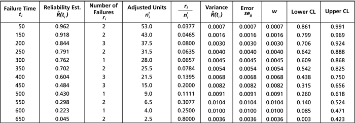
Once again, this type of problem is most readily solved by constructing a table similar to the following:
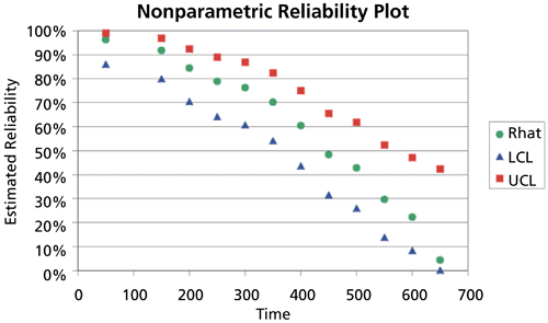
The following plot illustrates these results graphically:


