|
|
| (251 intermediate revisions by 10 users not shown) |
| Line 1: |
Line 1: |
| {{template:LDABOOK|8|The Weibull Distribution}} | | {{template:LDABOOK|8|The Weibull Distribution}} |
| | | The Weibull distribution is one of the most widely used lifetime distributions in reliability engineering. It is a versatile distribution that can take on the characteristics of other types of distributions, based on the value of the shape parameter, <math> {\beta} \,\!</math>. This chapter provides a brief background on the Weibull distribution, presents and derives most of the applicable equations and presents examples calculated both manually and by using ReliaSoft's [https://www.hbkworld.com/en/products/software/analysis-simulation/reliability/weibull-life-data-analysis-software Weibull++ software]. |
| =The Weibull Distribution=
| |
| | |
| The Weibull distribution is one of the most widely used lifetime distributions in reliability engineering. It is a versatile distribution that can take on the characteristics of other types of distributions, based on the value of the shape parameter, <math> \boldsymbol{\beta} </math>. This chapter provides a brief background on the Weibull distribution, presents and derives most of the applicable equations and presents examples calculated both manually and by using ReliaSoft's Weibull++. | |
|
| |
|
| == Weibull Probability Density Function == | | == Weibull Probability Density Function == |
| | ===The 3-Parameter Weibull=== |
| | {{three-parameter weibull distribution}} |
|
| |
|
| === The Three-Parameter Weibull Distribution === | | ===The 2-Parameter Weibull === |
| | | The 2-parameter Weibull ''pdf'' is obtained by setting |
| The three-parameter Weibull ''pdf'' is given by:
| |
| | |
| :::<math> f(T)={ \frac{\beta }{\eta }}\left( {\frac{T-\gamma }{\eta }}\right) ^{\beta -1}e^{-\left( {\frac{T-\gamma }{\eta }}\right) ^{\beta }} </math>
| |
| | |
| where,
| |
| | |
| ::::<math> f(T)\geq 0,\text{ }T\geq 0\text{ or }\gamma, </math>
| |
| | |
| ::::<math>\beta>0\ \,\!</math>,
| |
| | |
| ::::<math> \eta > 0 \,\!</math>,
| |
| | |
| ::::<math> -\infty < \gamma < +\infty \,\!</math>
| |
| | |
| and,
| |
| | |
| | |
| :::::<math> \eta= \,\!</math> scale parameter, or characteristic life
| |
| :::::<math> \beta= \,\!</math> shape parameter (or slope),
| |
| :::::<math> \gamma= \,\!</math> location parameter (or failure free life).
| |
| | |
| === The Two-Parameter Weibull Distribution ===
| |
| | |
| The two-parameter Weibull ''pdf'' is obtained by setting | |
| <math> \gamma=0 \,\!</math>, and is given by: | | <math> \gamma=0 \,\!</math>, and is given by: |
|
| |
|
| :::<math> f(T)={ \frac{\beta }{\eta }}\left( {\frac{T}{\eta }}\right) ^{\beta -1}e^{-\left( { \frac{T}{\eta }}\right) ^{\beta }} \,\!</math>
| | :<math> f(t)={ \frac{\beta }{\eta }}\left( {\frac{t}{\eta }}\right) ^{\beta -1}e^{-\left( { \frac{t}{\eta }}\right) ^{\beta }} \,\!</math> |
| | |
| === The One-Parameter Weibull Distribution ===
| |
|
| |
|
| The one-parameter Weibull ''pdf'' is obtained by again setting | | === The 1-Parameter Weibull=== |
| | The 1-parameter Weibull ''pdf'' is obtained by again setting |
| <math>\gamma=0 \,\!</math> and assuming <math>\beta=C=Constant \,\!</math> assumed value or: | | <math>\gamma=0 \,\!</math> and assuming <math>\beta=C=Constant \,\!</math> assumed value or: |
|
| |
|
| :::<math> f(T)={ \frac{C}{\eta }}\left( {\frac{T}{\eta }}\right) ^{C-1}e^{-\left( {\frac{T}{ \eta }}\right) ^{C}} \,\!</math>
| | ::<math> f(t)={ \frac{C}{\eta }}\left( {\frac{t}{\eta }}\right) ^{C-1}e^{-\left( {\frac{t}{ \eta }}\right) ^{C}} \,\!</math> |
|
| |
|
| where the only unknown parameter is the scale parameter, <math>\eta\,\!</math>. | | where the only unknown parameter is the scale parameter, <math>\eta\,\!</math>. |
|
| |
|
| Note that in the formulation of the one-parameter Weibull, we assume that the shape parameter <math>\beta \,\!</math> is known ''a priori'' from past experience on identical or similar products. The advantage of doing this is that data sets with few or no failures can be analyzed. | | Note that in the formulation of the 1-parameter Weibull, we assume that the shape parameter <math>\beta \,\!</math> is known ''a priori'' from past experience with identical or similar products. The advantage of doing this is that data sets with few or no failures can be analyzed. |
| | |
| == Weibull Statistical Properties ==
| |
| | |
| === The Mean or MTTF ===
| |
| | |
| The mean, <math> \overline{T} \,\!</math>, (also called ''MTTF'' of the Weibull ''pdf'' is given by:
| |
| | |
| :::<math> \overline{T}=\gamma +\eta \cdot \Gamma \left( {\frac{1}{\beta }}+1\right) \,\!</math>
| |
| | |
| where
| |
| :::<math> \Gamma \left( {\frac{1}{\beta }}+1\right) \,\!</math>
| |
| is the gamma function evaluated at the value of
| |
| :::<math> \left( { \frac{1}{\beta }}+1\right) \,\!</math>.
| |
| | |
| The gamma function is defined as:
| |
| | |
| :::<math> \Gamma (n)=\int_{0}^{\infty }e^{-x}x^{n-1}dx \,\!</math>
| |
| | |
| For the two-parameter case, this can be reduced to:
| |
| | |
| :::<math> \overline{T}=\eta \cdot \Gamma \left( {\frac{1}{\beta }}+1\right) \,\!</math>
| |
| | |
| Note that some practitioners erroneously assume that <math> \eta \,\!</math> is equal to the MTTF, <math> \overline{T}\,\!</math>.
| |
| This is only true for the case of
| |
| <math> \beta=1 \,\!</math> or
| |
| | |
| | |
| :::<math>
| |
| \begin{align}
| |
| \overline{T} &= \eta \cdot \Gamma \left( {\frac{1}{1}}+1\right) \\
| |
| &= \eta \cdot \Gamma \left( {\frac{1}{1}}+1\right) \\
| |
| &= \eta \cdot \Gamma \left( {2}\right) \\
| |
| &= \eta \cdot 1\\
| |
| &= \eta
| |
| \end{align}
| |
| </math>
| |
| | |
| === The Median ===
| |
| | |
| The median, <math> \breve{T}, </math> of the Weibull distribution is given by:
| |
| | |
| :::<math> \breve{T}=\gamma +\eta \left( \ln 2\right) ^{\frac{1}{\beta }} </math>
| |
| | |
| === The Mode ===
| |
| | |
| The mode, <math> \tilde{T}, </math> is given by:
| |
| | |
| :::<math> \tilde{T}=\gamma +\eta \left( 1-\frac{1}{\beta }\right) ^{\frac{1}{\beta }} </math>
| |
| | |
| === The Standard Deviation ===
| |
| | |
| The standard deviation, <span class="texhtml">σ<sub>''T''</sub>,</span> is given by:
| |
| | |
| :::<math> \sigma _{T}=\eta \cdot \sqrt{\Gamma \left( {\frac{2}{\beta }}+1\right) -\Gamma \left( {\frac{1}{ \beta }}+1\right) ^{2}} </math>
| |
| | |
| === The Weibull Reliability Function ===
| |
| | |
| The equation for the three-parameter Weibull cumulative density function, ''cdf'', is given by:
| |
| | |
| :::<math> F(T)=1-e^{-\left( \frac{T-\gamma }{\eta }\right) ^{\beta }} </math>.
| |
| | |
| This is also referred to as ''Unreliability'' and deignated as <math> Q(T) \,\!</math> by some authors.
| |
|
| |
| | |
| Recalling that the reliability function of a distribution is simply one minus the cdf, the reliability function for the three-parameter Weibull distribution is then given by:
| |
| | |
| :::<math> R(T)=e^{-\left( { \frac{T-\gamma }{\eta }}\right) ^{\beta }} </math>
| |
| | |
| === The Weibull Conditional Reliability Function ===
| |
| | |
| The three-parameter Weibull conditional reliability function is given by:
| |
| | |
| :::<math> R(t|T)={ \frac{R(T+t)}{R(T)}}={\frac{e^{-\left( {\frac{T+t-\gamma }{\eta }}\right) ^{\beta }}}{e^{-\left( {\frac{T-\gamma }{\eta }}\right) ^{\beta }}}} </math>
| |
|
| |
| or:
| |
| | |
| :::<math> R(t|T)=e^{-\left[ \left( {\frac{T+t-\gamma }{\eta }}\right) ^{\beta }-\left( {\frac{T-\gamma }{\eta }}\right) ^{\beta }\right] } </math>
| |
|
| |
|
| These gives the reliability for a new mission of <math> t \,\!</math> duration, having already accumulated <math> T \,\!</math> time of operation up to the start of this new mission, and the units are checked out to assure that they will start the next mission successfully. It is called conditional because you can calculate the reliability of a new mission based on the fact that the unit or units already accumulated hours of operation successfully.
| | ==Weibull Distribution Functions== |
| | | {{:Weibull Distribution Functions}} |
| === The Weibull Reliable Life ===
| |
| | |
| The reliable life, <math> T_{R} \,\!</math>, of a unit for a specified reliability,<math> R \,\!</math>, starting the mission at age zero, is given by:
| |
| | |
| :::<math> T_{R}=\gamma +\eta \cdot \left\{ -\ln ( R ) \right\} ^{ \frac{1}{\beta }} </math>
| |
| | |
| This is the life for which the unit/item will be functioning successfully with a reliability of <math> R \,\!</math>, . If ,<math> R=0.50 \,\!</math>, then <math> T_{R}=\breve{T} </math>, the median life, or the life by which half of the units will survive.
| |
| | |
| === The Weibull Failure Rate Function ===
| |
| | |
| The Weibull failure rate function, <math> \lambda(t) \,\!</math>, is given by:
| |
| | |
| :::<math> \lambda \left( T\right) = \frac{f\left( T\right) }{R\left( T\right) }=\frac{\beta }{\eta }\left( \frac{ T-\gamma }{\eta }\right) ^{\beta -1} </math>
| |
|
| |
|
| == Characteristics of the Weibull Distribution == | | == Characteristics of the Weibull Distribution == |
| | {{:Weibull Distribution Characteristics}} |
|
| |
|
| As was mentioned previously, the Weibull distribution is widely used in reliability and life data analysis due to its versatility. Depending on the values of the parameters, the Weibull distribution can be used to model a variety of life behaviors. We will now examine how the values of the shape parameter, <span class="texhtml">β</span>, and the scale parameter, <span class="texhtml">η</span>, affect such distribution characteristics as the shape of the curve, the reliability and the failure rate. Note that in the rest of this section we will assume the most general form of the Weibull distribution, i.e. the three-parameter form. The appropriate substitutions to obtain the other forms, such as the two-parameter form where <span class="texhtml">γ = 0,</span> or the one-parameter form where <span class="texhtml">β = ''C'' = </span>constant, can easily be made.
| | == Weibull Distribution Examples == |
| | | {{:Weibull Distribution Examples}} |
| === Characteristic Effects of the Shape Parameter, <span class="texhtml">β</span> ===
| |
| | |
| The Weibull shape parameter, <span class="texhtml">β</span>, is also known as the ''slope''. This is because the value of <span class="texhtml">β</span> is equal to the slope of the regressed line in a probability plot. Different values of the shape parameter can have marked effects on the behavior of the distribution. In fact, some values of the shape parameter will cause the distribution equations to reduce to those of other distributions. For example, when <span class="texhtml">β = 1</span>, the of the three-parameter Weibull reduces to that of the two-parameter exponential distribution or:
| |
| | |
| ::<math> f(T)={\frac{1}{\eta }}e^{-{\frac{T-\gamma }{\eta }}} </math>
| |
| | |
| where <math> \frac{1}{\eta }=\lambda = </math> failure rate. The parameter <span class="texhtml">β</span> is a pure number, i.e. it is dimensionless.
| |
| | |
| ==== The Effect of <span class="texhtml">β</span> on the <math>pdf</math> ====
| |
| | |
| Figure 6-1 shows the effect of different values of the shape parameter, <span class="texhtml">β</span>, on the shape of the <math>pdf</math>. One can see that the shape of the can take on a variety of forms based on the value of <span class="texhtml">β</span>.
| |
| | |
| [[Image:lda6.1.gif|thumb|center|600px| The effect of the Weibull shape parameter on the <math>pdf</math>.]]
| |
| | |
| | |
| For <math> 0<\beta \leq 1 </math>:
| |
| | |
| *As <span class="texhtml">''T''→0</span> <span class="texhtml">(</span>or <span class="texhtml">γ),</span> <span class="texhtml">''f''(''T'')→∞.</span>
| |
| | |
| *As <span class="texhtml">''T''→∞</span>, <span class="texhtml">''f''(''T'')→0</span>.
| |
| | |
| *<span class="texhtml">''f''(''T'')</span> decreases monotonically and is convex as increases beyond the value of <span class="texhtml">γ</span>.
| |
| | |
| *The mode is non-existent.
| |
| | |
| For <span class="texhtml">β > 1</span>:
| |
| | |
| *<span class="texhtml">''f''(''T'') = 0</span> at <span class="texhtml">(</span>or <span class="texhtml">γ)</span>.
| |
| | |
| *<span class="texhtml">''f''(''T'')</span> increases as <math> T\rightarrow \tilde{T} </math> (the mode) and decreases thereafter.
| |
| | |
| *For <span class="texhtml">β < 2.6</span> the Weibull <math>pdf</math> is positively skewed (has a right tail), for <span class="texhtml">2.6 < β < 3.7</span> its coefficient of skewness approaches zero (no tail). Consequently, it may approximate the normal <math>pdf</math> , and for <span class="texhtml">β > 3.7</span> it is negatively skewed (left tail). The way the value of <span class="texhtml">β</span> relates to the physical behavior of the items being modeled becomes more apparent when we observe how its different values affect the reliability and failure rate functions. Note that for <span class="texhtml">β = 0.999</span>, <span class="texhtml">''f''(0) = ∞</span>, but for <span class="texhtml">β = 1.001</span>, <span class="texhtml">''f''(0) = 0.</span> This abrupt shift is what complicates MLE estimation when <span class="texhtml">β</span> is close to one.
| |
| | |
| ==== The Effect of <span class="texhtml">β</span> on the <math>cdf</math> and Reliability Function ====
| |
| | |
| [[Image:lda6.2.gif|thumb|center|600px| Effect on <math>\beta</math> on the <math>cdf</math> on the Weibull probability plot with a fixed value of <math>\eta</math> ]]
| |
|
| |
| | |
| Figure 6-2 shows the effect of the value of <span class="texhtml">β</span> on the <math>cdf</math>, as manifested in the Weibull probability plot. It is easy to see why this parameter is sometimes referred to as the slope. Note that the models represented by the three lines all have the same value of <span class="texhtml">η</span>. Figure 6-3 shows the effects of these varied values of <span class="texhtml">β</span> on the reliability plot, which is a linear analog of the probability plot.
| |
| | |
| | |
| [[Image:lda6.3.gif|thumb|center|600px| The effect of values of <math>\beta</math> on the Weibull reliability plot. ]]
| |
| | |
| <br>
| |
| | |
| *<span class="texhtml">''R''(''T'')</span> decreases sharply and monotonically for <span class="texhtml">0 < β < 1</span> and is convex.
| |
| *For <span class="texhtml">β = 1</span>, <span class="texhtml">''R''(''T'')</span> decreases monotonically but less sharply than for <span class="texhtml">0 < β < 1</span> and is convex.
| |
| *For <span class="texhtml">β > 1</span>, <span class="texhtml">''R''(''T'')</span> decreases as increases. As wear-out sets in, the curve goes through an inflection point and decreases sharply.
| |
| | |
| <br>
| |
| | |
| ==== The Effect of <span class="texhtml">β</span> on the Weibull Failure Rate ====
| |
| | |
| The value of <span class="texhtml">β</span> has a marked effect on the failure rate of the Weibull distribution and inferences can be drawn about a population's failure characteristics just by considering whether the value of <span class="texhtml">β</span> is less than, equal to, or greater than one.
| |
| | |
| | |
| [[Image:lda6.4.gif|thumb|center|600px| The effect of <math>\beta</math> on the Weibull failure rate function. ]]
| |
| | |
| | |
| As indicated by Figure 6-4, populations with <span class="texhtml">β < 1</span> exhibit a failure rate that decreases with time, populations with <span class="texhtml">β = 1</span> have a constant failure rate (consistent with the exponential distribution) and populations with <span class="texhtml">β > 1</span> have a failure rate that increases with time. All three life stages of the bathtub curve can be modeled with the Weibull distribution and varying values of <span class="texhtml">β.</span> The Weibull failure rate for <span class="texhtml">0 < β < 1</span> is unbounded at <span class="texhtml">(</span>or <span class="texhtml">γ)</span>. The failure rate, <span class="texhtml">λ(''T''),</span> decreases thereafter monotonically and is convex, approaching the value of zero as <span class="texhtml">''T''→∞</span> or <span class="texhtml">λ(∞) = 0</span>. This behavior makes it suitable for representing the failure rate of units exhibiting early-type failures, for which the failure rate decreases with age. When encountering such behavior in a manufactured product, it may be indicative of problems in the production process, inadequate burn-in, substandard parts and components, or problems with packaging and shipping. For <span class="texhtml">β = 1</span>, <span class="texhtml">λ(''T'')</span> yields a constant value of <math> { \frac{1}{\eta }} </math> or:
| |
| | |
| ::<math> \lambda (T)=\lambda ={\frac{1}{\eta }} </math>
| |
| | |
| This makes it suitable for representing the failure rate of chance-type failures and the useful life period failure rate of units.
| |
| | |
| For <span class="texhtml">β > 1</span>, <span class="texhtml">λ(''T'')</span> increases as increases and becomes suitable for representing the failure rate of units exhibiting wear-out type failures. For <span class="texhtml">1 < β < 2,</span> the <span class="texhtml">λ(''T'')</span> curve is concave, consequently the failure rate increases at a decreasing rate as increases.
| |
| | |
| For <span class="texhtml">β = 2</span> there emerges a straight line relationship between <span class="texhtml">λ(''T'')</span> and , starting at a value of <span class="texhtml">λ(''T'') = 0</span> at <span class="texhtml">''T'' = γ</span>, and increasing thereafter with a slope of <math> { \frac{2}{\eta ^{2}}} </math>. Consequently, the failure rate increases at a constant rate as increases. Furthermore, if <span class="texhtml">η = 1</span> the slope becomes equal to 2, and when <span class="texhtml">γ = 0</span>, <span class="texhtml">λ(''T'')</span> becomes a straight line which passes through the origin with a slope of 2. Note that at <span class="texhtml">β = 2</span>, the Weibull distribution equations reduce to that of the Rayleigh distribution.
| |
| | |
| When <span class="texhtml">β > 2,</span> the <span class="texhtml">λ(''T'')</span> curve is convex, with its slope increasing as increases. Consequently, the failure rate increases at an increasing rate as increases indicating wear-out life.
| |
| | |
| <br>
| |
| | |
| === Characteristic Effects of the Scale Parameter, <span class="texhtml">η</span> ===
| |
| | |
| | |
| [[Image:lda6.5.gif|thumb|center|600px| The effects of <math>\eta</math> on the Weibull <math>pdf</math> for a common <math>\beta</math>. ]]
| |
|
| |
| | |
| A change in the scale parameter <span class="texhtml">η</span> has the same effect on the distribution as a change of the abscissa scale. Increasing the value of <span class="texhtml">η</span> while holding <span class="texhtml">β</span> constant has the effect of stretching out the . Since the area under a curve is a constant value of one, the "peak" of the pdf curve will also decrease with the increase of <span class="texhtml">η</span>, as indicated in Figure 6-5.
| |
| | |
| *If <span class="texhtml">η</span> is increased while <span class="texhtml">β</span> and <span class="texhtml">γ</span> are kept the same, the distribution gets stretched out to the right and its height decreases, while maintaining its shape and location.
| |
| | |
| *If <span class="texhtml">η</span> is decreased while <span class="texhtml">β</span> and <span class="texhtml">γ</span> are kept the same, the distribution gets pushed in towards the left (i.e. towards its beginning or towards 0 or <span class="texhtml">γ</span>), and its height increases.
| |
| | |
| *<span class="texhtml">η</span> has the same units as , such as hours, miles, cycles, actuations, etc.
| |
| | |
| <br>
| |
| | |
| === Characteristic Effects of the Location Parameter, <span class="texhtml">γ</span> ===
| |
| | |
| The location parameter, <span class="texhtml">γ</span>, as the name implies, locates the distribution along the abscissa. Changing the value of <span class="texhtml">γ</span> has the effect of ''sliding'' the distribution and its associated function either to the right (if <span class="texhtml">γ > 0</span>) or to the left (if <span class="texhtml">γ < 0</span>).''
| |
| | |
| | |
| [[Image:lda6.6.gif|thumb|center|600px| The effect of a positive location parameter, <math>\gamma</math>, on the position of the Weibull <math>pdf</math>. ]]
| |
| | |
| | |
| *When <span class="texhtml">γ = 0,</span> the distribution starts at or at the origin.
| |
| | |
| *If <span class="texhtml">γ > 0,</span> the distribution starts at the location <span class="texhtml">γ</span> to the right of the origin.
| |
| | |
| *If <span class="texhtml">γ < 0,</span> the distribution starts at the location <span class="texhtml">γ</span> to the left of the origin.
| |
| | |
| *<span class="texhtml">γ</span> provides an estimate of the earliest time-to-failure of such units.
| |
| | |
| *The life period 0 to <span class="texhtml">+ γ</span> is a failure free operating period of such units.
| |
| | |
| *The parameter <span class="texhtml">γ</span> may assume all values and provides an estimate of the earliest time a failure may be observed. A negative <span class="texhtml">γ</span> may indicate that failures have occurred prior to the beginning of the test, namely during production, in storage, in transit, during checkout prior to the start of a mission, or prior to actual use.
| |
| | |
| *<span class="texhtml">γ</span> has the same units as T, such as hours, miles, cycles, actuations, etc.
| |
| | |
| == Estimation of the Weibull Parameters ==
| |
| | |
| The estimates of the parameters of the Weibull distribution can be found graphically via probability plotting paper, or analytically, either using least squares or maximum likelihood.
| |
| | |
| === Probability Plotting ===
| |
| | |
| One method of calculating the parameters of the Weibull distribution is by using probability plotting. To better illustrate this procedure, consider the following example from Kececioglu [20].
| |
| | |
| ==== Example 1 ====
| |
| | |
| Assume that six identical units are being reliability tested at the same application and operation stress levels. All of these units fail during the test after operating the following number of hours, <span class="texhtml">''T''<sub>''i''</sub></span>: 93, 34, 16, 120, 53 and 75. Estimate the values of the parameters for a two-parameter Weibull distribution and determine the reliability of the units at a time of 15 hours.
| |
| | |
| ===== Solution to Example 1 =====
| |
| | |
| The steps for determining the parameters of the Weibull representing the data, using probability plotting, are outlined in the following instructions. First, rank the times-to-failure in ascending order as shown next.
| |
| | |
| {| border="1" cellspacing="0" cellpadding="5" align="center" | |
| |-
| |
| ! valign="middle" scope="col" align="center" | Time-to-failure, <br>hrs
| |
| ! valign="middle" scope="col" align="center" | Failure Order Number <br>out of Sample Size of 6
| |
| |-
| |
| | valign="middle" align="center" | 16
| |
| | valign="middle" align="center" | 1
| |
| |-
| |
| | valign="middle" align="center" | 34
| |
| | valign="middle" align="center" | 2
| |
| |-
| |
| | valign="middle" align="center" | 53
| |
| | valign="middle" align="center" | 3
| |
| |-
| |
| | valign="middle" align="center" | 75
| |
| | valign="middle" align="center" | 4
| |
| |-
| |
| | valign="middle" align="center" | 93
| |
| | valign="middle" align="center" | 5
| |
| |-
| |
| | valign="middle" align="center" | 120
| |
| | valign="middle" align="center" | 6
| |
| |}
| |
| | |
| Obtain their median rank plotting positions. Median rank positions are used instead of other ranking methods because median ranks are at a specific confidence level (50%). Median ranks can be found tabulated in many reliability books. They can also be estimated using the following equation,
| |
| | |
| ::<math> MR \sim { \frac{i-0.3}{N+0.4}}\cdot 100, </math>
| |
| | |
| where <math>i</math> is the failure order number and <math>N</math> is the total sample size. The exact median ranks are found in Weibull++ by solving,
| |
| | |
| ::<math>\sum_{k=i}^N{\binom{N}{k}}{MR^k}{(1-MR)^{N-k}}=0.5=50%
| |
| </math>
| |
| | |
| <br>for <math>MR</math>, where <math>N</math> is the sample size and <math>i</math> the order number. The times-to-failure, with their corresponding median ranks, are shown next.
| |
| | |
| {|align="center" border="1" cellspacing="1"
| |
| |-
| |
| | Time-to-failure, hrs
| |
| | Median Rank,%
| |
| |-
| |
| | 16
| |
| | 10.91
| |
| |-
| |
| | 34
| |
| | 26.44
| |
| |-
| |
| | 53
| |
| | 42.14
| |
| |-
| |
| | 75
| |
| | 57.86
| |
| |-
| |
| | 93
| |
| | 73.56
| |
| |-
| |
| | 120
| |
| | 89.1
| |
| |}
| |
| | |
| <br>
| |
| | |
| On a Weibull probability paper, plot the times and their corresponding ranks. A sample of a Weibull probability paper is given in Figure 6-7 and the plot of the data in the example in Figure 6-8.
| |
| | |
| | |
| [[Image:lda6.7.gif|thumb|center|600px| Example of Weibull probability plotting paper. ]]
| |
|
| |
| | |
| Draw the best possible straight line through these points, as shown below, then obtain the slope of this line by drawing a line, parallel to the one just obtained, through the slope indicator. This value is the estimate of the shape parameter <math> \hat{\beta } </math>, in this case <math> \hat{\beta }=1.4 </math>.
| |
| | |
| | |
| [[Image:lda6.8.gif|thumb|center|600px| Probability plot of data in Example 1.]]
| |
| | |
| | |
| At the <math> Q(t)=63.2% </math> ordinate point, draw a straight horizontal line until this line intersects the fitted straight line. Draw a vertical line through this intersection until it crosses the abscissa. The value at the intersection of the abscissa is the estimate of <math> \hat{\eta } </math>. For this case, <math> \hat{\eta }=76 </math> hours. (This is always at 63.2% since: <math> Q(T)=1-e^{-(\frac{\eta }{\eta })^{\beta }}=1-e^{-1}=0.632=63.2% </math>.
| |
| | |
| Now any reliability value for any mission time <math>t</math> can be obtained. For example, the reliability for a mission of 15 hours, or any other time, can now be obtained either from the plot or analytically. To obtain the value from the plot, draw a vertical line from the abscissa, at hours, to the fitted line. Draw a horizontal line from this intersection to the ordinate and read <span class="texhtml">''Q''(''t'')</span>, in this case <math> Q(t)=9.8% </math>. Thus, <math> R(t)=1-Q(t)=90.2% </math>. This can also be obtained analytically from the Weibull reliability function since the estimates of both of the parameters are known or:
| |
| | |
| <br><math> R(t=15)=e^{-\left( \frac{15}{\eta }\right) ^{\beta }}=e^{-\left( \frac{15}{76 }\right) ^{1.4}}=90.2% </math>
| |
| | |
| ==== Probability Plotting for the Location Parameter, <span class="texhtml">γ</span> ====
| |
| | |
| The third parameter of the Weibull distribution is utilized when the data do not fall on a straight line, but fall on either a concave up or down curve. The following statements can be made regarding the value of <span class="texhtml">γ:</span>
| |
| | |
| ''Case 1'': If the curve for MR versus <span class="texhtml">''T''<sub>''j''</sub></span> is concave down and the curve for MR versus <span class="texhtml">(''T''<sub>''j''</sub> − ''T''<sub>1</sub>)</span> is concave up, then there exists a <span class="texhtml">γ</span> such that <span class="texhtml">0 < γ < ''T''<sub>1</sub></span>, or <span class="texhtml">γ</span> has a positive value.
| |
| | |
| ''Case 2'': If the curves for MR versus <span class="texhtml">''T''<sub>''j''</sub></span> and MR versus <span class="texhtml">(''T''<sub>''j''</sub> − ''T''<sub>1</sub>)</span> are both concave up, then there exists a negative <span class="texhtml">γ</span> which will straighten out the curve of MR versus <span class="texhtml">''T''<sub>''j''</sub></span>.
| |
| | |
| ''Case 3'': If neither one of the previous two cases prevails, then either reject the Weibull as one capable of representing the data, or proceed with the multiple population (mixed Weibull) analysis. To obtain the location parameter, <span class="texhtml">γ:</span>
| |
| | |
| *Subtract the same arbitrary value, <span class="texhtml">γ</span>, from all the times to failure and replot the data.
| |
| | |
| *If the initial curve is concave up, subtract a negative <span class="texhtml">γ</span> from each failure time.
| |
| | |
| *If the initial curve is concave down, subtract a positive <span class="texhtml">γ</span> from each failure time.
| |
| | |
| *Repeat until the data plots on an acceptable straight line.
| |
| | |
| *The value of <span class="texhtml">γ</span> is the subtracted (positive or negative) value that places the points in an acceptable straight line.
| |
| | |
| | |
| The other two parameters are then obtained using the techniques previously described. Also, it is important to note that we used the term subtract a positive or negative gamma, where subtracting a negative gamma is equivalent to adding it. Note that when adjusting for gamma, the x-axis scale for the straight line becomes <span class="texhtml">(''T'' − γ).</span>
| |
| | |
| ===Example 2===
| |
| | |
| Six identical units are reliability tested under the same stresses and conditions. All units are tested to failure and the following times-to-failure are recorded: 48, 66, 85, 107, 125 and 152 hours. Find the parameters of the three-parameter Weibull distribution using probability plotting.
| |
| | |
| ==== Solution to Example 2 ====
| |
| | |
| The following figure shows the results. Note that since the original data set was concave down, 17.26 was subtracted from all the times-to-failure and replotted, resulting in a straight line, thus <span class="texhtml">γ = 17.26</span>. (We used Weibull++ to get the results. To perform this by hand, one would attempt different values of <span class="texhtml">γ,</span> using a trial and error methodology, until an acceptable straight line is found. When performed manually, you do not expect decimal accuracy.)
| |
| | |
| <br>
| |
| | |
| [[Image:lda6.9.gif|thumb|center|600px|]]
| |
| | |
| === Rank Regression on Y ===
| |
| | |
| Performing rank regression on Y requires that a straight line mathematically be fitted to a set of data points such that the sum of the squares of the vertical deviations from the points to the line is minimized. This is in essence the same methodology as the probability plotting method, except that we use the principle of least squares to determine the line through the points, as opposed to just eyeballing it. The first step is to bring our function into a linear form. For the two-parameter Weibull distribution, the (cumulative density function) is:
| |
| | |
| ::<math> F(T)=1-e^{-\left( \frac{T}{\eta }\right) ^{\beta }} (Fw) </math>
| |
| | |
| Taking the natural logarithm of both sides of the equation yields:
| |
| | |
| ::<math>\ln[ 1-F(T)] =-( \frac{T}{\eta }) ^{\beta } </math>
| |
| | |
| ::<math> \ln{ -\ln[ 1-F(T)]} =\beta \ln ( \frac{T}{ \eta }) </math>
| |
| | |
| or:
| |
| | |
| ::<math> \ln \{ -\ln[ 1-F(T)]\} =-\beta \ln (\eta )+\beta \ln (T) EQNREF logw </math>
| |
| | |
| Now let:
| |
| | |
| ::<math> y = \ln \{ -\ln[ 1-F(T)]\} ( yw )</math>
| |
| | |
| ::<math> a = − βln(\eta) </math> (aw)
| |
| | |
| and:
| |
| | |
| ::<math> b= \beta</math> ( bw )
| |
| | |
| which results in the linear equation of:
| |
| | |
| ::<math>y=a+bx</math>
| |
| | |
| The least squares parameter estimation method (also known as regression analysis) was discussed in Chapter 3 and the following equations for regression on Y were derived in Appendix A:
| |
| | |
| ::<math> \hat{a}=\frac{\sum\limits_{i=1}^{N}y_{i}}{N}-\hat{b}\frac{ \sum\limits_{i=1}^{N}x_{i}}{N}=\bar{y}-\hat{b}\bar{x} EQNREF aaw </math>
| |
| | |
| and:
| |
| | |
| ::<math> \hat{b}={\frac{\sum\limits_{i=1}^{N}x_{i}y_{i}-\frac{\sum \limits_{i=1}^{N}x_{i}\sum\limits_{i=1}^{N}y_{i}}{N}}{\sum \limits_{i=1}^{N}x_{i}^{2}-\frac{\left( \sum\limits_{i=1}^{N}x_{i}\right) ^{2}}{N}}} EQNREF bbw </math>
| |
| | |
| In this case the equations for <span class="texhtml">''y''<sub>''i''</sub></span> and <span class="texhtml">''x''<sub>''i''</sub></span> are:
| |
| | |
| ::<math> y_{i}=\ln \left\{ -\ln [1-F(T_{i})]\right\} , </math>
| |
| | |
| and:
| |
| | |
| ::<span class="texhtml">''x''<sub>''i''</sub> = ln(''T''<sub>''i''</sub>).</span>
| |
| | |
| The <math> F(T_{i})^{\prime }s </math> are estimated from the median ranks.
| |
| | |
| Once <math> \hat{a} </math> and <math> \hat{b} </math> are obtained, then <math> \hat{\beta } </math> and <math> \hat{\eta } </math> can easily be obtained from Eqns. (EQNREF aw ) and (\ref {bw}).
| |
| | |
| ==== The Correlation Coefficient ====
| |
| | |
| The correlation coefficient is defined as follows:
| |
| | |
| ::<math> \rho ={\frac{\sigma _{xy}}{\sigma _{x}\sigma _{y}}} </math>
| |
| | |
| where, <span class="texhtml">σ<sub>''x'' ''y''</sub> = </span>covariance of and , <span class="texhtml">σ<sub>''x''</sub> = </span>standard deviation of , and <span class="texhtml">σ<sub>''y''</sub> = </span>standard deviation of . The estimator of <span class="texhtml">ρ</span> is the sample ''correlation coefficient'', <math> \hat{\rho} </math>, given by:
| |
| | |
| ::<math> \hat{\rho}=\frac{\sum\limits_{i=1}^{N}(x_{i}-\overline{x})(y_{i}-\overline{y} )}{\sqrt{\sum\limits_{i=1}^{N}(x_{i}-\overline{x})^{2}\cdot \sum\limits_{i=1}^{N}(y_{i}-\overline{y})^{2}}} EQNREF RHOw </math>
| |
| | |
| <br>
| |
| | |
| ===== Example 3 =====
| |
| | |
| Consider the data in Example 1, where six units were tested to failure and the following failure times were recorded: 16, 34, 53, 75, 93 and 120 hours. Estimate the parameters and the correlation coefficient using rank regression on Y, assuming that the data follow the two-parameter Weibull distribution.
| |
| | |
| ===== Solution to Example 3 =====
| |
| | |
| Construct a table as shown below.
| |
| | |
| {|align="center" border=1 cellspacing=1
| |
| |+ Table 6.1 - Least Squares Analysis
| |
| |-
| |
| | N||<math>T_{i}</math>||<math>ln(T_{i})</math>|| <math>F(T_i)</math>||<math>y_{i}</math>||<math>(ln{T_i})^2</math>||<math>{y_i}^2</math>||<math>(ln{T_i})y_i</math>
| |
| |-
| |
| |1 ||16||2.7726||0.1091||-2.1583||7.6873||4.6582||-5.9840
| |
| |-
| |
| |2 ||34||3.5264||0.2645||-1.1802||12.4352||1.393||-4.1620
| |
| |-
| |
| |3 ||53||3.9703||0.4214||-0.6030||15.7632||0.3637||-2.3943
| |
| |-
| |
| |4 ||75||4.3175||0.5786||-0.146||18.6407||0.0213||-0.6303
| |
| |-
| |
| |5 ||93||4.5326||0.7355||0.2851||20.5445||0.0813||1.2923
| |
| |-
| |
| |6 ||120||4.7875||0.8909||0.7955||22.9201||0.6328||3.8083
| |
| |-
| |
| |<math>\sum</math>|| ||23.9068|| ||-3.007||97.9909||7.1502||-8.0699
| |
| |}
| |
| | |
| | |
| Utilizing the values from Table 6.1, calculate <math> \hat{a} </math> and <math> \hat{b} </math> using Eqns. (EQNREF aaw ) and (EQNREF bbw );
| |
| <math> \hat{b} =\frac{\sum\limits_{i=1}^{6}(\ln T_{i})y_{i}-(\sum\limits_{i=1}^{6}\ln T_{i})(\sum\limits_{i=1}^{6}y_{i})/6}{ \sum\limits_{i=1}^{6}(\ln T_{i})^{2}-(\sum\limits_{i=1}^{6}\ln T_{i})^{2}/6}
| |
| </math>
| |
| | |
| ::<math> \hat{b}=\frac{-8.0699-(23.9068)(-3.0070)/6}{97.9909-(23.9068)^{2}/6} </math>
| |
| | |
| or
| |
| | |
| ::<math> \hat{b}=1.4301 </math>
| |
| | |
| and:
| |
| | |
| ::<math> \hat{a}=\overline{y}-\hat{b}\overline{T}=\frac{\sum \limits_{i=1}^{N}y_{i}}{N}-\hat{b}\frac{\sum\limits_{i=1}^{N}\ln T_{i}}{N } </math>
| |
| | |
| or:
| |
| | |
| ::<math> \hat{a}=\frac{(-3.0070)}{6}-(1.4301)\frac{23.9068}{6}=-6.19935 </math>
| |
| | |
| Therefore, from Eqn. (EQNREF bw ):
| |
| | |
| ::<math> \hat{\beta }=\hat{b}=1.4301 </math>
| |
| | |
| and from Eqn. (EQNREF aw ):
| |
| | |
| ::<math> \hat{\eta }=e^{-\frac{\hat{a}}{\hat{b}}}=e^{-\frac{(-6.19935)}{ 1.4301}} </math>
| |
| | |
| or:
| |
| | |
| ::<math> \hat{\eta }=76.318\text{ hr} </math>
| |
| | |
| The correlation coefficient can be estimated using Eqn. (EQNREF RHOw ):
| |
| | |
| ::<math> \hat{\rho }=0.9956 </math>
| |
| | |
| The above example can be repeated using Weibull++. Start Weibull++ and create a new ''Data Folio''.
| |
| | |
| [[Image:datafolioicon.gif|thumb|center|300px|]]
| |
| | |
| Select the '' Times-to-failure data'' option.
| |
| | |
| | |
| [[Image:newdatasheetsetup.gif|thumb|center|600px| The effect of the Weibull shape parameter on the <math>pdf</math>. ]]
| |
| | |
| | |
| Enter the times-to-failure in the datasheet (ignore the Subset ID column), as shown next. The times-to-failure need not be sorted, Weibull++ will automatically sort the data.
| |
| | |
| <br>
| |
| [[Image:ldachp6fig1.gif|thumb|center|600px| ]]
| |
| | |
| | |
| Select the desired method of analysis. Note that we are assuming that the underlying distribution is the Weibull, so make sure that the Weibull distribution is selected. Under ''Parameters/Type'' on the Main page, select ''2''.
| |
| | |
| <br>
| |
| [[Image:ldachp6fig2.gif|thumb|center|600px|]]
| |
| | |
| | |
| Also, so that you get the same results as this example, switch to the ''Analysis'' page and make sure you are using the ''Rank Regression on Y (RRY)'' calculation method with this example, as shown next.
| |
| | |
| [[Image:ldachp6fig3.gif|thumb|center|600px| ]]
| |
| | |
| Note that this can also be done from the ''Main'' page by clicking the left bottom box under the Results area. Each time you click that box you will see the method switch between MLE, RRX, and RRY. Click the ''Calculate'' icon,
| |
| | |
| [[Image:calculateicon.gif|thumb|center|600px|]]
| |
|
| |
| | |
| or select ''Calculate'' from the ''Data'' menu. The results will appear in the Data Folio's ''Results area''. The next figure shows the results for this example.
| |
| | |
| [[Image:ldachp6fig4.gif|thumb|center|600px| ]]
| |
| | |
| <br>
| |
| You can now plot the results by clicking the ''Plot'' icon,
| |
| | |
| [[Image:ploticon.gif|thumb|center|600px| ]]
| |
| | |
| or by selecting ''Plot Probability'' from the ''Data'' menu.
| |
| | |
| The Weibull probability plot for these data is shown next.
| |
| | |
| The confidence bounds, as determined from the Fisher matrix, can also be plotted. Select ''Confidence Bounds'' from the ''Plot'' menu, choose ''Two-Sided'' under ''Sides,'' ''Reliability (Type II)'' under ''Type'' and enter ''90'' for the ''Confidence level.
| |
| | |
| [[Image:confidenceboundssetup.gif|thumb|center|600px| ]]
| |
|
| |
| | |
| The plot will appear as follows,
| |
| | |
| [[Image:ldachp6fig5.gif|thumb|center|600px| ]]
| |
| | |
| If desired, the Weibull <math>pdf</math> representing these data can be written as:
| |
| | |
| ::<math> f(T)={\frac{\beta }{\eta }}\left( {\frac{T}{\eta }}\right) ^{\beta -1}e^{-\left( {\frac{T}{\eta }}\right) ^{\beta }} </math>
| |
| | |
| or:
| |
| | |
| ::<math> f(T)={\frac{1.4302}{76.317}}\left( {\frac{T}{76.317}}\right) ^{0.4302}e^{-\left( {\frac{T}{76.317}}\right) ^{1.4302}} </math> You can also plot the Weibull by selecting ''Pdf Plot'' from the ''Plot Type'' drop-down menu on the control panel to the right of the plot area.
| |
| | |
| [[Image:ldachp6fig6.gif|thumb|center|600px| ]]
| |
| | |
| | |
| From this point on, different results, reports and plots can be obtained.
| |
| | |
| === Rank Regression on X ===
| |
| | |
| Performing a rank regression on X is similar to the process for rank regression on Y, with the difference being that the ''horizontal'' deviations from the points to the line are minimized rather than the vertical. Again, the first task is to bring our function, Eqn. (EQNREF Fw ), into a linear form. This step is exactly the same as in the regression on Y analysis and Eqns. (EQNREF logw ), (EQNREF yw ), (EQNREF aw ) and (EQNREF bw ) apply in this case too. The derivation from the previous analysis begins on the least squares fit part, where in this case we treat as the dependent variable and as the independent variable. The best-fitting straight line to the data, for regression on X (see Chapter 3), is the straight line:
| |
| | |
| ::<math> x= \hat{a}+\hat{b}y </math> EQNREF xlinew
| |
| | |
| The corresponding equations for <math> \hat{a} </math> and <math> \hat{b} </math> are:
| |
| | |
| ::<math> \hat{a}=\overline{x}-\hat{b}\overline{y}=\frac{\sum\limits_{i=1}^{N}x_{i}}{N} -\hat{b}\frac{\sum\limits_{i=1}^{N}y_{i}}{N} </math>
| |
| | |
| and
| |
| | |
| ::<math> \hat{b}={\frac{\sum\limits_{i=1}^{N}x_{i}y_{i}-\frac{\sum \limits_{i=1}^{N}x_{i}\sum\limits_{i=1}^{N}y_{i}}{N}}{\sum \limits_{i=1}^{N}y_{i}^{2}-\frac{\left( \sum\limits_{i=1}^{N}y_{i}\right) ^{2}}{N}}} </math>
| |
| | |
| where:
| |
| | |
| ::<math> y_{i}=\ln \left\{ -\ln [1-F(T_{i})]\right\} </math> and:
| |
| | |
| <span class="texhtml">''x''<sub>''i''</sub> = ln(''T''<sub>''i''</sub>)</span> and the <span class="texhtml">''F''(''T''<sub>''i''</sub>)</span> values are again obtained from the median ranks.
| |
| | |
| Once <math> \hat{a} </math> and <math> \hat{b} </math> are obtained, solve Eqn. (EQNREF xlinew ) for <span class="texhtml">''y'',</span> which corresponds to:
| |
| | |
| ::<math> y=-\frac{\hat{a}}{\hat{b}}+\frac{1}{\hat{b}}x </math> Solving for the parameters from Eqns. (EQNREF aw ) and (EQNREF bw ) we get
| |
| | |
| ::<math> a=-\frac{\hat{a}}{\hat{b}}=-\beta \ln (\eta )</math> EQNREF awx
| |
| | |
| and
| |
| | |
| ::<math> b=\frac{1}{\hat{b}}=\beta EQNREF bwx </math> The correlation coefficient is evaluated as before using Eqn. (EQNREF RHOw ).
| |
| | |
| ==== Example 4 ====
| |
| | |
| Repeat Example 1 using rank regression on X.
| |
| | |
| ===== Solution to Example 4 =====
| |
| | |
| Solution to Example 4 Table 6.1, constructed in Example 3, can also be applied to this example.
| |
| | |
| Using the values from this table we get:
| |
| | |
| ::<math> \hat{b} ={\frac{\sum\limits_{i=1}^{6}(\ln T_{i})y_{i}-\frac{ \sum\limits_{i=1}^{6}\ln T_{i}\sum\limits_{i=1}^{6}y_{i}}{6}}{ \sum\limits_{i=1}^{6}y_{i}^{2}-\frac{\left( \sum\limits_{i=1}^{6}y_{i}\right) ^{2}}{6}}}
| |
| </math>
| |
| | |
| ::<math>\hat{b} =\frac{-8.0699-(23.9068)(-3.0070)/6}{7.1502-(-3.0070)^{2}/6} </math>
| |
| | |
| or:
| |
| | |
| ::<math> \hat{b}=0.6931 </math>
| |
| | |
| and:
| |
| | |
| ::<math> \hat{a}=\overline{x}-\hat{b}\overline{y}=\frac{\sum\limits_{i=1}^{6}\ln T_{i} }{6}-\hat{b}\frac{\sum\limits_{i=1}^{6}y_{i}}{6} </math>
| |
| | |
| or:
| |
| | |
| ::<math> \hat{a}=\frac{23.9068}{6}-(0.6931)\frac{(-3.0070)}{6}=4.3318 </math>
| |
| | |
| Therefore, from Eqn. (EQNREF bwx ):
| |
| | |
| ::<math> \hat{\beta }=\frac{1}{\hat{b}}=\frac{1}{0.6931}=1.4428 </math>
| |
| | |
| and from Eqn. (EQNREF awx )
| |
| | |
| ::<math> \hat{\eta }=e^{\frac{\hat{a}}{\hat{b}}\cdot \frac{1}{\hat{ \beta }}}=e^{\frac{4.3318}{0.6931}\cdot \frac{1}{1.4428}}=76.0811\text{ hr} </math>
| |
| | |
| The correlation coefficient is found using Eqn. (EQNREF RHOw ):
| |
| | |
| ::<math> \hat{\rho }=0.9956 </math>
| |
| | |
| The results and the associated graph using Weibull++ are given next. Note that the slight variation in the results is due to the number of significant figures used in the estimation of the median ranks. Weibull++ by default uses double precision accuracy when computing the median ranks.
| |
| | |
| | |
| [[Image:ldachp6fig7.gif|thumb|center|600px| ]]
| |
| | |
| <br>
| |
| | |
| === Three-Parameter Weibull Regression ===
| |
| | |
| When the MR versus <span class="texhtml">''T''<sub>''j''</sub></span> points plotted on the Weibull probability paper do not fall on a satisfactory straight line and the points fall on a curve,(Note that other shapes, particularly shapes, might suggest the existence of more than one population. In these cases, the multiple population, mixed Weibull distribution, may be more appropriate. Chapter 10 presents the mixed Weibull distribution.) then a location parameter, <span class="texhtml">γ</span>, might exist which may straighten out these points. The goal in this case is to fit a curve, instead of a line, through the data points using nonlinear regression. The Gauss-Newton method can be used to solve for the parameters, <span class="texhtml">β</span>, <span class="texhtml">η</span> and <span class="texhtml">γ</span>, by performing a Taylor series expansion on <span class="texhtml">''F''(''T''<sub>''i''</sub>;β,η,γ)</span>. Then the nonlinear model is approximated with linear terms and ordinary least squares are employed to estimate the parameters. This procedure is iterated until a satisfactory solution is reached. Weibull++ 7 calculates the value of <span class="texhtml">γ</span> by utilizing an optimized Nelder-Mead algorithm, and adjusts the points by this value of <span class="texhtml">γ</span> such that they fall on a straight line, and then plots both the adjusted and the original unadjusted points. To draw a curve through the original unadjusted points, if so desired, select Weibull 3P Line Unadjusted for Gamma from the ''Show Plot Line'' submenu under the ''Plot Options'' menu. The returned estimations of the parameters are the same when selecting RRX or RRY. To display the unadjusted data points and line along with the adjusted data points and line, select ''Show/Hide Items'' under the ''Plot Options ''menu and include the unadjusted data points and line as follows:
| |
| | |
| [[Image:ldashowhideplotitems.gif|thumb|center|600px| ]]
| |
| | |
| The results and the associated graph for the previous example using the three-parameter Weibull case are shown next:
| |
| | |
| [[Image:preMLE.gif|thumb|center|600px| ]]
| |
| <br>
| |
| | |
| === Maximum Likelihood Estimation ===
| |
| | |
| As outlined in Chapter 3, maximum likelihood estimation works by developing a likelihood function based on the available data and finding the values of the parameter estimates that maximize the likelihood function. This can be achieved by using iterative methods to determine the parameter estimate values that maximize the likelihood function, but this can be rather difficult and time-consuming, particularly when dealing with the three-parameter distribution. Another method of finding the parameter estimates involves taking the partial derivatives of the likelihood function with respect to the parameters, setting the resulting equations equal to zero and solving simultaneously to determine the values of the parameter estimates. ( Note that MLE asymptotic properties do not hold when estimating <span class="texhtml">γ</span> using MLE [27].) The log-likelihood functions and associated partial derivatives used to determine maximum likelihood estimates for the Weibull distribution are covered in Appendix C.
| |
| | |
| | |
| ====Example 5====
| |
| Repeat Example 1 using maximum likelihood estimation.
| |
| | |
| | |
| =====Solution to Example 5=====
| |
| In this case, we have non-grouped data with no suspensions or intervals, i.e. complete data. The equations for the partial derivatives of the log-likelihood function are derived in Appendix C and given next:
| |
| | |
| ::<math> \frac{\partial \Lambda }{\partial \beta }=\frac{6}{\beta } +\sum_{i=1}^{6}\ln \left( \frac{T_{i}}{\eta }\right) -\sum_{i=1}^{6}\left( \frac{T_{i}}{\eta }\right) ^{\beta }\ln \left( \frac{T_{i}}{\eta }\right) =0
| |
| </math>
| |
| | |
| and:
| |
| | |
| ::<math> \frac{\partial \Lambda }{\partial \eta }=\frac{-\beta }{\eta }\cdot 6+\frac{ \beta }{\eta }\sum\limits_{i=1}^{6}\left( \frac{T_{i}}{\eta }\right) ^{\beta }=0 </math>
| |
| | |
| Solving the above equations simultaneously we get:
| |
| | |
| ::<math> \hat{\beta }=1.933,</math> <math>\hat{\eta }=73.526 </math>
| |
| | |
| <br>
| |
| The variance/covariance matrix is found to be,
| |
| | |
| ::<math> \left[ \begin{array}{ccc} \hat{Var}\left( \hat{\beta }\right) =0.4211 & \hat{Cov}( \hat{\beta },\hat{\eta })=3.272 \\
| |
| | |
| \hat{Cov}(\hat{\beta },\hat{\eta })=3.272 & \hat{Var} \left( \hat{\eta }\right) =266.646 \end{array} \right] </math>
| |
| | |
| | |
| The results and the associated graph using Weibull++ (MLE) are shown next.
| |
| | |
| [[File:ex5folio.gif|center]]
| |
| | |
| You can view the variance/covariance matrix directly by clicking the ''Quick Calculation Pad ''(QCP) icon
| |
| | |
| [[File:qcpicon.gif|center]]
| |
| | |
| and then clicking the ''Show Fisher Matrix'' button on the ''Confidence Bounds'' tab of the QCP.
| |
| | |
| [[File:ex5qcp.gif|center]]
| |
| | |
| [[File:ex5folio2.gif|center]]
| |
| | |
| <br> Note that the decimal accuracy displayed and used is based on your individual User Setup.
| |
| | |
| == Fisher Matrix Confidence Bounds ==
| |
| | |
| One of the methods used by the application in estimating the different types of confidence bounds for Weibull data, the Fisher matrix method, is presented in this section. The complete derivations were presented in detail (for a general function) in Chapter 5.
| |
| | |
| === Bounds on the Parameters ===
| |
| | |
| One of the properties of maximum likelihood estimators is that they are asymptotically normal, meaning that for large samples they are normally distributed. Additionally, since both the shape parameter estimate, <math> \hat{\beta } </math>, and the scale parameter estimate, <math> \hat{\eta }, </math> must be positive, thus <span class="texhtml">lnβ</span> and <span class="texhtml">lnη</span> are treated as being normally distributed as well. The lower and upper bounds on the parameters are estimated from [30]:
| |
| | |
| ::<math> \beta _{U} =\hat{\beta }\cdot e^{\frac{K_{\alpha }\sqrt{Var(\hat{ \beta })}}{\hat{\beta }}}\text{ (upper bound)} </math>
| |
| | |
| ::<math> \beta _{L} =\frac{\hat{\beta }}{e^{\frac{K_{\alpha }\sqrt{Var(\hat{ \beta })}}{\hat{\beta }}}} \text{ (lower bound)}
| |
| </math>
| |
| | |
| and:
| |
| | |
| ::<math> \eta _{U} =\hat{\eta }\cdot e^{\frac{K_{\alpha }\sqrt{Var(\hat{ \eta })}}{\hat{\eta }}}\text{ (upper bound)}
| |
| </math>
| |
| | |
| ::<math> \eta _{L} =\frac{\hat{\eta }}{e^{\frac{K_{\alpha }\sqrt{Var(\hat{ \eta })}}{\hat{\eta }}}}\text{ (lower bound)} </math>
| |
| | |
| where <math> K_{\alpha}</math> is defined by:
| |
| | |
| ::<math> \alpha =\frac{1}{\sqrt{2\pi }}\int_{K_{\alpha }}^{\infty }e^{-\frac{t^{2}}{2} }dt=1-\Phi (K_{\alpha }) </math>
| |
| | |
| If <span class="texhtml">δ</span> is the confidence level, then <math> \alpha =\frac{1-\delta }{2} </math> for the two-sided bounds and <span class="texhtml">α = 1 − δ</span> for the one-sided bounds. The variances and covariances of <math> \hat{\beta } </math> and <math> \hat{\eta } </math> are estimated from the inverse local Fisher matrix, as follows:
| |
|
| |
| | |
| ::<math> \left( \begin{array}{cc} \hat{Var}\left( \hat{\beta }\right) & \hat{Cov}\left( \hat{ \beta },\hat{\eta }\right)
| |
| \\
| |
| \hat{Cov}\left( \hat{\beta },\hat{\eta }\right) & \hat{Var} \left( \hat{\eta }\right) \end{array} \right) =\left( \begin{array}{cc} -\frac{\partial ^{2}\Lambda }{\partial \beta ^{2}} & -\frac{\partial ^{2}\Lambda }{\partial \beta \partial \eta }
| |
| \\
| |
| | |
| -\frac{\partial ^{2}\Lambda }{\partial \beta \partial \eta } & -\frac{ \partial ^{2}\Lambda }{\partial \eta ^{2}} \end{array} \right) _{\beta =\hat{\beta },\text{ }\eta =\hat{\eta }}^{-1} </math>
| |
| | |
| | |
| ===Fisher Matrix Confidence Bounds and Regression Analysis===
| |
| | |
| Note that the variance and covariance of the parameters are obtained from the inverse Fisher information matrix as described in this section. The local Fisher information matrix is obtained from the second partials of the likelihood function, by substituting the solved parameter estimates into the particular functions. This method is based on maximum likelihood theory and is derived from the fact that the parameter estimates were computed using maximum likelihood estimation methods. When one uses least squares or regression analysis for the parameter estimates, this methodology is theoretically then not applicable. However, if one assumes that the variance and covariance of the parameters will be similar ( One also assumes similar properties for both estimators.) regardless of the underlying solution method, then the above methodology can also be used in regression analysis.
| |
| | |
| The Fisher matrix is one of the methodologies that Weibull++ uses for both MLE and regression analysis. Specifically, Weibull++ uses the likelihood function and computes the local Fisher information matrix based on the estimates of the parameters and the current data. This gives consistent confidence bounds regardless of the underlying method of solution, i.e. MLE or regression. In addition, Weibull++ checks this assumption and proceeds with it if it considers it to be acceptable. In some instances, Weibull++ will prompt you with an "Unable to Compute Confidence Bounds" message when using regression analysis. This is an indication that these assumptions were violated.
| |
| | |
| === Bounds on Reliability ===
| |
| | |
| The bounds on reliability can easily be derived by first looking at the general extreme value distribution (EVD). Its reliability function is given by:
| |
| | |
| ::<math> R(t)=e^{-e^{\left( \frac{t-p_{1}}{p_{2}}\right) }} </math>
| |
| | |
| By transforming <span class="texhtml">''t'' = ln''T''</span> and converting <math> p=\ln{\eta}</math>, <math> p_{2}=\frac{1}{ \beta } </math>, the above equation becomes the Weibull reliability function:
| |
| | |
| ::<math> R(T)=e^{-e^{\beta \left( \ln T-\ln \eta \right) }}=e^{-e^{\ln \left( \frac{T }{\eta }\right) ^{\beta }}}=e^{-\left( \frac{T}{\eta }\right) ^{\beta }} </math> With:
| |
| | |
| ::<math> R(T)=e^{-e^{\beta \left( \ln T-\ln \eta \right) }} EQNREF eq27 </math>
| |
| | |
| set <math> u=\beta \left( \ln T-\ln \eta \right). </math> The reliability function now becomes:
| |
| | |
| ::<math> R(T)=e^{-e^{u}} </math>
| |
| | |
| The next step is to find the upper and lower bounds on <span class="texhtml">''u''.</span> Using the equations derived in Chapter 5, the bounds on are then estimated from [30]:
| |
| | |
| ::<math> u_{U} =\hat{u}+K_{\alpha }\sqrt{Var(\hat{u})}
| |
| </math>
| |
| | |
| ::<math> u_{L} =\hat{u}-K_{\alpha }\sqrt{Var(\hat{u})}
| |
| </math>
| |
| | |
| where:
| |
| | |
| ::<math> Var(\hat{u}) =\left( \frac{\partial u}{\partial \beta }\right) ^{2}Var( \hat{\beta })+\left( \frac{\partial u}{\partial \eta }\right) ^{2}Var( \hat{\eta }) +2\left( \frac{\partial u}{\partial \beta }\right) \left( \frac{\partial u }{\partial \eta }\right) Cov\left( \hat{\beta },\hat{\eta }\right) </math>
| |
| | |
| or:
| |
| | |
| ::<math> Var(\hat{u}) =\frac{\hat{u}^{2}}{\hat{\beta }^{2}}Var(\hat{ \beta })+\frac{\hat{\beta }^{2}}{\hat{\eta }^{2}}Var(\hat{\eta }) -\left( \frac{2u}{\hat{\eta }}\right) Cov\left( \hat{\beta }, \hat{\eta }\right). EQNREF eq32
| |
| | |
| </math>
| |
| | |
| The upper and lower bounds on reliability are:
| |
| | |
| ::<math> R_{U} =e^{-e^{u_{L}}}\text{ (upper bound)}</math>
| |
| | |
| ::<math> R_{L} =e^{-e^{u_{U}}}\text{ (lower bound)}</math>
| |
| | |
| ==== Other Weibull Forms ====
| |
| | |
| Weibull++ makes the following assumptions/substitutions in Eqn. (EQNREF eq27 ) to Eqn. (EQNREF eq32 ) when using the three-parameter or one-parameter forms:
| |
| | |
| *For the three-parameter case, substitute <math> t=\ln (T-\hat{\gamma }) </math> (and by definition <span class="texhtml">γ < ''T''</span>)<span class="texhtml">,</span> instead of <span class="texhtml">ln''T''.</span> (Note that this is an approximation since it eliminates the third parameter and assumes that <math> Var( \hat{\gamma })=0. </math>)
| |
| | |
| *For the one-parameter, <math> Var(\hat{\beta })=0, </math> thus:
| |
| | |
| ::<math> Var(\hat{u})=\left( \frac{\partial u}{\partial \eta }\right) ^{2}Var( \hat{\eta })=\left( \frac{\hat{\beta }}{\hat{\eta }}\right) ^{2}Var(\hat{\eta }) </math>
| |
| | |
| Also note that the time axis (x-axis) in the three-parameter Weibull plot in Weibull++ 7 is not but <span class="texhtml">''T'' − γ.</span> This means that one must be cautious when obtaining confidence bounds from the plot. If one desires to estimate the confidence bounds on reliability for a given time <span class="texhtml">''T''<sub>0</sub></span> from the adjusted plotted line, then these bounds should be obtained for a <span class="texhtml">''T''<sub>0</sub> − γ</span> entry on the time axis.
| |
| | |
| === Bounds on Time ===
| |
| | |
| The bounds around the time estimate or reliable life estimate, for a given Weibull percentile (unreliability), are estimated by first solving the reliability equation with respect to time, as follows [24, 30]:
| |
| | |
| ::<math> \ln R =-\left( \frac{T}{\eta }\right) ^{\beta }
| |
| </math>
| |
| | |
| ::<math> \ln (-\ln R) =\beta \ln \left( \frac{T}{\eta }\right) </math>
| |
| | |
| ::<math> \ln (-\ln R) =\beta (\ln T-\ln \eta )</math>
| |
| | |
| or:
| |
| | |
| ::<math> u=\frac{1}{\beta }\ln (-\ln R)+\ln \eta </math>
| |
| | |
| where <span class="texhtml">''u'' = ln''T''.</span>
| |
| | |
| The upper and lower bounds on are estimated from:
| |
| | |
| ::<math> u_{U} =\hat{u}+K_{\alpha }\sqrt{Var(\hat{u})} </math>
| |
| | |
| ::<math> u_{L} =\hat{u}-K_{\alpha }\sqrt{Var(\hat{u})} </math>
| |
| | |
| where:
| |
| | |
| ::<math> Var(\hat{u})=\left( \frac{\partial u}{\partial \beta }\right) ^{2}Var( \hat{\beta })+\left( \frac{\partial u}{\partial \eta }\right) ^{2}Var( \hat{\eta })+2\left( \frac{\partial u}{\partial \beta }\right) \left( \frac{\partial u}{\partial \eta }\right) Cov\left( \hat{\beta },\hat{ \eta }\right) </math>
| |
| | |
| or:
| |
| ::<math> Var(\hat{u}) =\frac{1}{\hat{\beta }^{4}}\left[ \ln (-\ln R)\right] ^{2}Var(\hat{\beta })+\frac{1}{\hat{\eta }^{2}}Var(\hat{\eta })+2\left( -\frac{1}{\hat{\beta }^{2}}\right) \left( \frac{\ln (-\ln R)}{ \hat{\eta }}\right) Cov\left( \hat{\beta },\hat{\eta }\right) </math>
| |
| | |
| The upper and lower bounds are then found by:
| |
| | |
| ::<math> T_{U} =e^{u_{U}}\text{ (upper bound)} </math>
| |
| | |
| ::<math> T_{L} =e^{u_{L}}\text{ (lower bound)} </math>
| |
| | |
| == Likelihood Ratio Confidence Bounds ==
| |
| | |
| As covered in Chapter 5, the likelihood confidence bounds are calculated by finding values for <span class="texhtml">θ<sub>1</sub></span> and <span class="texhtml">θ<sub>2</sub></span> that satisfy:
| |
| | |
| ::<math> -2\cdot \text{ln}\left( \frac{L(\theta _{1},\theta _{2})}{L(\hat{\theta }_{1}, \hat{\theta }_{2})}\right) =\chi _{\alpha ;1}^{2} EQNREF lratio2 </math>
| |
| | |
| This equation can be rewritten as:
| |
| | |
| ::<math> L(\theta _{1},\theta _{2})=L(\hat{\theta }_{1},\hat{\theta } _{2})\cdot e^{\frac{-\chi _{\alpha ;1}^{2}}{2}} EQNREF lratio3 </math>
| |
| | |
| For complete data, the likelihood function for the Weibull distribution is given by:
| |
| | |
| ::<math> L(\beta ,\eta )=\prod_{i=1}^{N}f(x_{i};\beta ,\eta )=\prod_{i=1}^{N}\frac{ \beta }{\eta }\cdot \left( \frac{x_{i}}{\eta }\right) ^{\beta -1}\cdot e^{-\left( \frac{x_{i}}{\eta }\right) ^{\beta }} </math>
| |
| | |
| For a given value of <span class="texhtml">α</span>, values for <span class="texhtml">β</span> and <span class="texhtml">η</span> can be found which represent the maximum and minimum values that satisfy Eqn. (\ref {lratio3}). These represent the confidence bounds for the parameters at a confidence level <span class="texhtml">δ</span>, where <span class="texhtml">α = δ</span> for two-sided bounds and <span class="texhtml">α = 2δ − 1</span> for one-sided.
| |
| | |
| Similarly, the bounds on time and reliability can be found by substituting the Weibull reliability equation into the likelihood function so that it is in terms of <span class="texhtml">β</span> and time or reliability, as discussed in Chapter 5. The likelihood ratio equation used to solve for bounds on time (Type 1) is:
| |
|
| |
| | |
| ::<math> L(\beta ,t)=\prod_{i=1}^{N}\frac{\beta }{\left( \frac{t}{(-\text{ln}(R))^{ \frac{1}{\beta }}}\right) }\cdot \left( \frac{x_{i}}{\left( \frac{t}{(-\text{ ln}(R))^{\frac{1}{\beta }}}\right) }\right) ^{\beta -1}\cdot \text{exp}\left[ -\left( \frac{x_{i}}{\left( \frac{t}{(-\text{ln}(R))^{\frac{1}{\beta }}} \right) }\right) ^{\beta }\right] </math>
| |
| | |
| The likelihood ratio equation used to solve for bounds on reliability (Type 2) is:
| |
| | |
| ::<math> L(\beta ,R)=\prod_{i=1}^{N}\frac{\beta }{\left( \frac{t}{(-\text{ln}(R))^{ \frac{1}{\beta }}}\right) }\cdot \left( \frac{x_{i}}{\left( \frac{t}{(-\text{ ln}(R))^{\frac{1}{\beta }}}\right) }\right) ^{\beta -1}\cdot \text{exp}\left[ -\left( \frac{x_{i}}{\left( \frac{t}{(-\text{ln}(R))^{\frac{1}{\beta }}} \right) }\right) ^{\beta }\right] </math>
| |
| | |
| == Bayesian Confidence Bounds ==
| |
| | |
| === Bounds on Parameters ===
| |
| | |
| Bayesian Bounds use non-informative prior distributions for both parameters. From Chapter 5, we know that if the prior distribution of <span class="texhtml">η</span> and <span class="texhtml">β</span> are independent, the posterior joint distribution of <span class="texhtml">η</span> and <span class="texhtml">β</span> can be written as:
| |
| | |
| ::<math> f(\eta ,\beta |Data)= \dfrac{L(Data|\eta ,\beta )\varphi (\eta )\varphi (\beta )}{\int_{0}^{\infty }\int_{0}^{\infty }L(Data|\eta ,\beta )\varphi (\eta )\varphi (\beta )d\eta d\beta } </math>
| |
| | |
| The marginal distribution of <span class="texhtml">η</span> is:
| |
| | |
| ::<math> f(\eta |Data) =\int_{0}^{\infty }f(\eta ,\beta |Data)d\beta =
| |
| \dfrac{\int_{0}^{\infty }L(Data|\eta ,\beta )\varphi (\eta )\varphi (\beta )d\beta }{\int_{0}^{\infty }\int_{-\infty }^{\infty }L(Data|\eta ,\beta )\varphi (\eta )\varphi (\beta )d\eta d\beta }
| |
| </math>
| |
| | |
| where: <math> \varphi (\beta )=\frac{1}{\beta } </math> is the non-informative prior of <span class="texhtml">β</span>. <math> \varphi (\eta )=\frac{1}{\eta } </math> is the non-informative prior of <span class="texhtml">η</span>. Using these non-informative prior distributions, <math>f(\eta|Data)</math> can be rewritten as:
| |
| | |
| ::<math> f(\eta |Data)=\dfrac{\int_{0}^{\infty }L(Data|\eta ,\beta )\frac{1}{\beta } \frac{1}{\eta }d\beta }{\int_{0}^{\infty }\int_{0}^{\infty }L(Data|\eta ,\beta )\frac{1}{\beta }\frac{1}{\eta }d\eta d\beta } </math>
| |
| | |
| The one-sided upper bounds of <span class="texhtml">η</span> is:
| |
| | |
| ::<math> CL=P(\eta \leq \eta _{U})=\int_{0}^{\eta _{U}}f(\eta |Data)d\eta </math>
| |
| | |
| The one-sided lower bounds of <span class="texhtml">η</span> is:
| |
| | |
| ::<math> 1-CL=P(\eta \leq \eta _{L})=\int_{0}^{\eta _{L}}f(\eta |Data)d\eta </math> The two-sided bounds of <span class="texhtml">η</span> is:
| |
| | |
| ::<math> CL=P(\eta _{L}\leq \eta \leq \eta _{U})=\int_{\eta _{L}}^{\eta _{U}}f(\eta |Data)d\eta </math> Same method is used to obtain the bounds of <span class="texhtml">β</span>.
| |
| | |
| === Bounds on Time (Type 1) ===
| |
| | |
| From Chapter 5, we know that:
| |
| | |
| ::<math> CL=\Pr (T\leq T_{U})=\Pr (\eta \leq T_{U}\exp (-\frac{\ln (-\ln R)}{\beta })) </math> From the posterior distribution of <span class="texhtml">η</span>, we have:
| |
| | |
| ::<math> CL=\dfrac{\int\nolimits_{0}^{\infty }\int\nolimits_{0}^{T_{U}\exp (-\dfrac{ \ln (-\ln R)}{\beta })}L(\beta ,\eta )\frac{1}{\beta }\frac{1}{\eta }d\eta d\beta }{\int\nolimits_{0}^{\infty }\int\nolimits_{0}^{\infty }L(\beta ,\eta )\frac{1}{\beta }\frac{1}{\eta }d\eta d\beta } EQNREF BayesCLT </math>
| |
| | |
| Eqn. (EQNREF BayesCLT ) is solved numerically for <span class="texhtml">''T''<sub>''U''</sub>.</span> The same method can be applied to calculate one sided lower bounds and two-sided bounds on time.
| |
| | |
| === Bounds on Reliability (Type 2) ===
| |
| | |
| ::<math> CL=\Pr (R\leq R_{U})=\Pr (\eta \leq T\exp (-\frac{\ln (-\ln R_{U})}{\beta })) </math> From the posterior distribution of <span class="texhtml">η,</span> we have:
| |
| | |
| ::<math> CL=\dfrac{\int\nolimits_{0}^{\infty }\int\nolimits_{0}^{T\exp (-\dfrac{\ln (-\ln R_{U})}{\beta })}L(\beta ,\eta )\frac{1}{\beta }\frac{1}{\eta }d\eta d\beta }{\int\nolimits_{0}^{\infty }\int\nolimits_{0}^{\infty }L(\beta ,\eta )\frac{1}{\beta }\frac{1}{\eta }d\eta d\beta } EQNREF BayesCLR </math>
| |
| | |
| Eqn. (EQNREF BayesCLR ) is solved numerically for <span class="texhtml">''R''<sub>''U''</sub>.</span> The same method can be used to calculate the one sided lower bounds and two-sided bounds on reliability.
| |
| | |
| == Weibull-Bayesian Analysis ==
| |
| | |
| In this section, the Bayesian methods are presented for the two-parameter Weibull distribution. Bayesian concepts were introduced in Chapter 3. This model considers prior knowledge on the shape (<span class="texhtml">β</span>) parameter of the Weibull distribution when it is chosen to be fitted to a given set of data. There are many practical applications for this model, particularly when dealing with small sample sizes and some prior knowledge for the shape parameter is available. For example, when a test is performed, there is often a good understanding about the behavior of the failure mode under investigation, primarily through historical data. At the same time, most reliability tests are performed on a limited number of samples. Under these conditions, it would be very useful to use this prior knowledge with the goal of making more accurate predictions. A common approach for such scenarios is to use the one-parameter Weibull distribution, but this approach is too deterministic, too absolute you may say (and you would be right). The Weibull-Bayesian model in Weibull++ (which is actually a true "WeiBayes" model, unlike the one-parameter Weibull that is commonly referred to as such) offers an alternative to the one-parameter Weibull, by including the variation and uncertainty that might have been observed in the past on the shape parameter. Applying Bayes's rule on the two-parameter Weibull distribution and assuming the prior distributions of <span class="texhtml">β</span> and <span class="texhtml">η</span> are independent, we obtain the following posterior :
| |
| | |
| ::<math> f(\beta ,\eta |Data)=\dfrac{L(\beta ,\eta )\varphi (\beta )\varphi (\eta )}{ \int\nolimits_{0}^{\infty }\int\nolimits_{0}^{\infty }L(\beta ,\eta )\varphi (\beta )\varphi (\eta )d\eta d\beta } </math> EQNREF WeibBayes
| |
| | |
| In this model, <span class="texhtml">η</span> is assumed to follow a noninformative prior distribution with the density function <math> \varphi (\eta )=\dfrac{1}{\eta } </math>. This is called Jeffrey's prior, and is obtained by performing a logarithmic transformation on <span class="texhtml">η.</span> Specifically, since <span class="texhtml">η</span> is always positive, we can assume that ln(<span class="texhtml">η)</span> follows a uniform distribution, <span class="texhtml">''U''( − ∞, + ∞).</span> Applying Jeffrey's rule [9] which says "in general, an approximate non-informative prior is taken proportional to the square root of Fisher's information", yields <math> \varphi (\eta )=\dfrac{1}{\eta }. </math>
| |
| | |
| The prior distribution of <span class="texhtml">β</span>, denoted as <math> \varphi (\beta ) </math>, can be selected from the following distributions: normal, lognormal, exponential and uniform. The procedure of performing a Weibull-Bayesian analysis is as follows:
| |
| | |
| *Collect the times-to-failure data.
| |
| | |
| *Specify a prior distribution for <span class="texhtml">β</span> (the prior for <span class="texhtml">η</span> is assumed to be 1/<span class="texhtml">η).</span>
| |
| | |
| *Obtain the posterior from Eqn. (EQNREF WeibBayes ).
| |
| | |
| In other words, a distribution (the posterior ) is obtained, rather than a point estimate as in classical statistics (i.e., as in the parameter estimation methods described previously in this chapter). Therefore, if a point estimate needs to be reported, a point of the posterior needs to be calculated. Typical points of the posterior distribution used are the mean (expected value) or median. In Weibull++, both options are available and can be chosen from the ''Analysis'' page, under the ''Results As'' area, as shown next.
| |
| | |
| [[File:resultsaschp6.gif|center]]
| |
| | |
| The expected value of <span class="texhtml">β</span> is obtained by:
| |
|
| |
| | |
| ::<math> E(\beta )=\int\nolimits_{0}^{\infty }\int\nolimits_{0}^{\infty }\beta \cdot f(\beta ,\eta |Data)d\beta d\eta </math>
| |
| | |
| Similarly, the expected value of <span class="texhtml">η</span> is obtained by:
| |
|
| |
| | |
| ::<math> E(\eta )=\int\nolimits_{0}^{\infty }\int\nolimits_{0}^{\infty }\eta \cdot f(\beta ,\eta |Data)d\beta d\eta </math>
| |
| | |
| The median points are obtained by solving the following equations for <math> \breve{\beta} </math> and <math> \breve{\eta} </math> respectively:
| |
| | |
| ::<math> \int\nolimits_{0}^{\infty }\int\nolimits_{0}^{\breve{\beta}}f(\beta ,\eta |Data)d\beta d\eta =0.5 </math>
| |
| | |
| and
| |
| | |
| ::<math> \int\nolimits_{0}^{\breve{\eta}}\int\nolimits_{0}^{\infty }f(\beta ,\eta |Data)d\beta d\eta =0.5 </math>
| |
| | |
| Of course, other points of the posterior distribution can be calculated as well. For example, one may want to calculate the 10th percentile of the joint posterior distribution (w.r.t. one of the parameters). The procedure for obtaining other points of the posterior distribution is similar to the one for obtaining the median values, where instead of 0.5 the percentage of interest is given. This procedure actually provides the confidence bounds on the parameters, which in the Bayesian framework are called ‘‘Credible Bounds‘‘. However, since the engineering interpretation is the same, and to avoid confusion, we refer to them as confidence bounds in this reference and in Weibull++.
| |
| | |
| === Posterior Distributions for Functions of Parameters ===
| |
| | |
| As explained in Chapter 3, in Bayesian analysis, all the functions of the parameters are distributed. In other words, a posterior distribution is obtained for functions such as reliability and failure rate, instead of point estimate as in classical statistics. Therefore, in order to obtain a point estimate for these functions, a point on the posterior distributions needs to be calculated. Again, the expected value (mean) or median value are used.
| |
| | |
| ====<math>pdf</math> of the Times-to-Failure ====
| |
| | |
| The posterior distribution of the failure time is given by:
| |
| | |
| <math> f(T|Data)=\int\nolimits_{0}^{\infty }\int\nolimits_{0}^{\infty }f(T,\beta ,\eta )f(\beta ,\eta |Data)d\eta d\beta </math> EQNREF WeibBayesPDF
| |
| | |
| where:
| |
| | |
| <math> f(T,\beta ,\eta )=\dfrac{\beta }{\eta }\left( \dfrac{T}{\eta }\right) ^{\beta -1}e^{-\left( \dfrac{T}{\eta }\right) ^{\beta }} </math>
| |
| | |
| For the <math>pdf</math> of the times-to-failure, only the expected value is calculated and reported in Weibull++.
| |
| | |
| ==== Reliability ====
| |
| | |
| In order to calculate the median value of the reliability function, we first need to obtain posterior of the reliability. Since <span class="texhtml">''R''(''T'')</span> is a function of <span class="texhtml">β</span>, the density functions of <span class="texhtml">β</span> and <span class="texhtml">''R''(''T'')</span> have the following relationship:
| |
| | |
| ::<math> \begin{align} f(R|Data,T)dR = & f(\beta |Data)d\beta)\\
| |
| = & (\int\nolimits_{0}^{\infty }f(\beta ,\eta |Data)d{\eta}) d{\beta} \\
| |
| =& \dfrac{\int\nolimits_{0}^{\infty }L(\beta ,\eta )\varphi (\beta )\varphi (\eta )d\eta }{\int\nolimits_{0}^{\infty }\int\nolimits_{0}^{\infty }L(\beta ,\eta )\varphi (\beta )\varphi (\eta )d\eta d\beta }d\beta
| |
| \end{align}
| |
| </math> EQNREF Rpdf
| |
| | |
| | |
| The median value of the reliability is obtained by solving the following equation w.r.t. <math> \breve{R}: </math>
| |
| | |
| ::<math> \int\nolimits_{0}^{\breve{R}}f(R|Data,T)dR=0.5 </math> EQNREF MedRel
| |
| | |
| The expected value of the reliability at time is given by:
| |
| | |
| ::<math> R(T|Data)=\int\nolimits_{0}^{\infty }\int\nolimits_{0}^{\infty }R(T,\beta ,\eta )f(\beta ,\eta |Data)d\eta d\beta </math> where:
| |
| | |
| ::<math> R(T,\beta ,\eta )=e^{-\left( \dfrac{T}{\eta }\right) ^{^{\beta }}} </math>
| |
| | |
| <br>
| |
| | |
| ==== Failure Rate ====
| |
| | |
| The failure rate at time is given by:
| |
| | |
| ::<math> \lambda (T|Data)=\dfrac{\int\nolimits_{0}^{\infty }\int\nolimits_{0}^{\infty }\lambda (T,\beta ,\eta )L(\beta ,\eta )\varphi (\eta )\varphi (\beta )d\eta d\beta }{\int\nolimits_{0}^{\infty }\int\nolimits_{0}^{\infty }L(\beta ,\eta )\varphi (\eta )\varphi (\beta )d\eta d\beta } </math>
| |
| | |
| where:
| |
| | |
| ::<math> \lambda (T,\beta ,\eta )=\dfrac{\beta }{\eta }\left( \dfrac{T}{\eta }\right) ^{\beta -1} </math>
| |
| | |
| <br>
| |
| | |
| === Note on Calculated Results ===
| |
| | |
| As mentioned above, in order to obtain point estimates for the parameters of functions of the parameters in Bayesian analysis, the Median or Mean values of the different posterior <math>pdf</math>s are calculated. It is important to note that the Median value is preferable and is the default in Weibull++. This is because the Median value always corresponds to the 50th percentile of the distribution. On the other hand, the Mean is not a fixed point on the distribution, which could cause issues, especially when comparing results across different data sets.
| |
| | |
| === Confidence Bounds on <span class="texhtml">''R''(''T'')</span> ===
| |
| | |
| The confidence bounds calculation under the Weibull-Bayesian analysis is very similar to the Bayesian Confidence Bounds method described in the previous section, with the exception that in the case of the Weibull-Bayesian Analysis the specified prior of <span class="texhtml">β</span> is considered instead of an non-informative prior. The Bayesian one-sided upper bound estimate for <span class="texhtml">''R''(''T'')</span> is given by:
| |
| | |
| ::<math> \int\nolimits_{0}^{R_{U}(T)}f(R|Data,T)dR=CL </math>
| |
| | |
| Using Eqns. (EQNREF WeibBayes ) and (EQNREF Rpdf ) the following is obtained:
| |
| | |
| ::<math> \dfrac{\int\nolimits_{0}^{\infty }\int\nolimits_{T\exp (-\dfrac{\ln (-\ln R_{U})}{\beta })}^{\infty }L(\beta ,\eta )\varphi (\beta )\varphi (\eta )d\eta d\beta }{\int\nolimits_{0}^{\infty }\int\nolimits_{0}^{\infty }L(\beta ,\eta )\varphi (\beta )\varphi (\eta )d\eta d\beta }=CL </math> EQNREF 1CLRU
| |
| | |
| Eqn. (EQNREF 1CLRU ) can be solved for <span class="texhtml">''R''<sub>''U''</sub>(''T'')</span>. The Bayesian one-sided lower bound estimate for <math> \ R(T) </math> is given by:
| |
| | |
| ::<math> \int\nolimits_{0}^{R_{L}(T)}f(R|Data,T)dR=1-CL </math>
| |
| | |
| Using Eqns. (EQNREF WeibBayes ) and (EQNREF Rpdf ) the following is obtained:
| |
| | |
| ::<math> \dfrac{\int\nolimits_{0}^{\infty }\int\nolimits_{0}^{T\exp (-\dfrac{\ln (-\ln R_{L})}{\beta })}L(\beta ,\eta )\varphi (\beta )\varphi (\eta )d\eta d\beta }{\int\nolimits_{0}^{\infty }\int\nolimits_{0}^{\infty }L(\beta ,\eta )\varphi (\beta )\varphi (\eta )d\eta d\beta }=1-CL </math> EQNREF 1CLRL
| |
| | |
| Eqn. (EQNREF 1CLRL ) can be solved for <span class="texhtml">''R''<sub>''L''</sub>(''T'')</span>. The Bayesian two-sided bounds estimate for <span class="texhtml">''R''(''T'')</span> is given by:
| |
| | |
| ::<math> \int\nolimits_{R_{L}(T)}^{R_{U}(T)}f(R|Data,T)dR=CL </math> which is equivalent to:
| |
| | |
| ::<math> \int\nolimits_{0}^{R_{U}(T)}f(R|Data,T)dR=(1+CL)/2 </math>
| |
| | |
| and
| |
| | |
| ::<math> \int\nolimits_{0}^{R_{L}(T)}f(R|Data,T)dR=(1-CL)/2 </math>
| |
| | |
| Using the same method for one-sided bounds, <span class="texhtml">''R''<sub>''U''</sub>(''T'')</span>and <span class="texhtml">''R''<sub>''L''</sub>(''T'')</span> can be computed.
| |
| | |
| === Confidence Bounds on Time <math>T</math> ===
| |
| | |
| Following the same procedure described for bounds on Reliability, the bounds of time can be calculated, given . The Bayesian one-sided upper bound estimate for <span class="texhtml">''T''(''R'')</span> is given by:
| |
| | |
| ::<math> \int\nolimits_{0}^{T_{U}(R)}f(T|Data,R)dT=CL </math>
| |
| | |
| Using Eqns. (EQNREF WeibBayes ) and. (EQNREF WeibBayesPDF ), we obtain:
| |
| | |
| ::<math> \dfrac{\int\nolimits_{0}^{\infty }\int\nolimits_{0}^{T_{U}\exp (-\dfrac{\ln (-\ln R)}{\beta })}L(\beta ,\eta )\varphi (\beta )\varphi (\eta )d\eta d\beta }{\int\nolimits_{0}^{\infty }\int\nolimits_{0}^{\infty }L(\beta ,\eta )\varphi (\beta )\varphi (\eta )d\eta d\beta }=CL </math> EQNREF 1CLTU
| |
| | |
| Eqn. (EQNREF 1CLTU ) can be solved for <span class="texhtml">''T''<sub>''U''</sub>(''R'')</span>. The Bayesian one-sided lower bound estimate for <span class="texhtml">''T''(''R'')</span> is given by:
| |
| | |
| ::<math> \int\nolimits_{0}^{T_{L}(R)}f(T|Data,R)dT=1-CL </math>
| |
| | |
| or:
| |
| | |
| ::<math> \dfrac{\int\nolimits_{0}^{\infty }\int\nolimits_{T_{L}\exp (\dfrac{-\ln (-\ln R)}{\beta })}^{\infty }L(\beta ,\eta )\varphi (\beta )\varphi (\eta )d\eta d\beta }{\int\nolimits_{0}^{\infty }\int\nolimits_{0}^{\infty }L(\beta ,\eta )\varphi (\beta )\varphi (\eta )d\eta d\beta }=CL </math> EQNREF 1CLTL
| |
| | |
| Eqn. (EQNREF 1CLTL ) can be solved for <span class="texhtml">''T''<sub>''L''</sub>(''R'')</span>. The Bayesian two-sided lower bounds estimate for <span class="texhtml">''T''(''R'')</span> is:
| |
| | |
| ::<math> \int\nolimits_{T_{L}(R)}^{T_{U}(R)}f(T|Data,R)dT=CL </math>
| |
| | |
| which is equivalent to:
| |
| | |
| ::<math> \int\nolimits_{0}^{T_{U}(R)}f(T|Data,R)dT=(1+CL)/2 </math>
| |
| | |
| and:
| |
| | |
| ::<math> \int\nolimits_{0}^{T_{L}(R)}f(T|Data,R)dT=(1-CL)/2 </math>
| |
| | |
| <br>
| |
| | |
| | |
| ====Example 6====
| |
| | |
| A manufacturer has tested prototypes of a modified product. The test was terminated at 2000 hours, with only two failures observed from a sample size of eighteen.
| |
| | |
| {| border=1 cellspacing=1 align="center"
| |
| |-
| |
| |Number of State||State of F or S||State End Time
| |
| |-
| |
| | 1 || F || 1180
| |
| |-
| |
| | 1 || F || 1842
| |
| |-
| |
| | 16 || S || 2000
| |
| |}
| |
| | |
| Because of the lack of failure data in the prototype testing, the manufacturer decided to use information gathered from prior tests on this product to increase the confidence in the results of the prototype testing. This decision was made because failure analysis indicated that the failure mode of these two failures is the same as the one observed in previous tests. In other words, it is expected that the shape of the distribution hasn't changed, but hopefully the scale has, indicating longer life. The two-parameter Weibull distribution have been used to model all prior tests results. The list of the estimated <span class="texhtml">β</span> parameter is as follows:
| |
| | |
| {| border=1 cellspacing=1 align="center"
| |
| |-
| |
| |Betas Obtained for Similar Mode
| |
| |-
| |
| | 1.7
| |
| |-
| |
| | 2.1
| |
| |-
| |
| | 2.4
| |
| |-
| |
| |3.1
| |
| |-
| |
| |3.5
| |
| |}
| |
| | |
| | |
| First, in order to fit the data to a Weibull-Bayesian model, a prior distribution for <span class="texhtml">β</span> needs to be determined. Based on the prior tests' <span class="texhtml">β</span> values, the prior distribution for <span class="texhtml">β</span> was found to be a lognormal distribution with <span class="texhtml">μ = 0.9064</span>, <span class="texhtml">σ = 0.3325</span> (obtained by entering the <span class="texhtml">β</span> values into a Weibull++ ''Standard Folio'' and analyzing it based on the RRX analysis method.)
| |
| | |
| the test data is entered into a ''Standard Folio'', the Weibull-Bayesian is selected under '' Distribution'' and the <span class="texhtml">β</span> prior distribution is entered after clicking the ''Calculate'' button.
| |
| | |
| [[File:chp6folio2data1.gif|center]]
| |
| | |
| Suppose that the reliability at 3000hr is the metric of interest in this example. This reliability can be obtained using Eqn. (EQNREF MedRel ), resulting in the median value of the posterior of the reliability at 3000hr. Using the ''QCP'', this value is calculated to be 76.97. ( By default Weibull++ returns the median values of the posterior distribution. )
| |
| | |
| The posterior <math>pdf</math> of the reliability function at 3000hrs can be obtained using Eqn. (EQNREF Rpdf ). In Figure 6-10 the posterior <math>pdf</math> of the reliability at 3000hrs is plotted, with the corresponding median value as well as the 10th percentile value shown. The 10th percentile constitutes the 90 Lower 1-Sided bound on the reliability at 3000hrs, which is calculated to be 50.77.
| |
| | |
| [[File:lda6.10.gif|center]]
| |
| | |
| Notice that the <math>pdf</math> plotted in Fig. 6-10 is of the reliability at 3000hrs, and not the <math>pdf</math> of the times-to-failure data. The <math>pdf</math> of the times-to-failure data can be obtained using Eqn. (EQNREF WeibBayesPDF ) and plotted using Weibull++, as shown next:
| |
| | |
| [[File:chp6plotofdata1.gif|center]]
| |
| | |
| | |
| <br>
| |
| {{RS Copyright}}
| |
| | |
| [[Category:Life_Data_Analysis_Reference]]
| |
New format available! This reference is now available in a new format that offers faster page load, improved display for calculations and images, more targeted search and the latest content available as a PDF. As of September 2023, this Reliawiki page will not continue to be updated. Please update all links and bookmarks to the latest reference at help.reliasoft.com/reference/life_data_analysis
|
Chapter 8: The Weibull Distribution
|
The Weibull distribution is one of the most widely used lifetime distributions in reliability engineering. It is a versatile distribution that can take on the characteristics of other types of distributions, based on the value of the shape parameter, [math]\displaystyle{ {\beta} \,\! }[/math]. This chapter provides a brief background on the Weibull distribution, presents and derives most of the applicable equations and presents examples calculated both manually and by using ReliaSoft's Weibull++ software.
Weibull Probability Density Function
The 3-Parameter Weibull
The 3-parameter Weibull pdf is given by:
- [math]\displaystyle{ f(t)={ \frac{\beta }{\eta }}\left( {\frac{t-\gamma }{\eta }}\right) ^{\beta -1}e^{-\left( {\frac{t-\gamma }{\eta }}\right) ^{\beta }} \,\! }[/math]
where:
- [math]\displaystyle{ f(t)\geq 0,\text{ }t\geq \gamma \,\! }[/math]
- [math]\displaystyle{ \beta\gt 0\ \,\! }[/math]
- [math]\displaystyle{ \eta \gt 0 \,\! }[/math]
- [math]\displaystyle{ -\infty \lt \gamma \lt +\infty \,\! }[/math]
and:
- [math]\displaystyle{ \eta= \,\! }[/math] scale parameter, or characteristic life
- [math]\displaystyle{ \beta= \,\! }[/math] shape parameter (or slope)
- [math]\displaystyle{ \gamma= \,\! }[/math] location parameter (or failure free life)
The 2-Parameter Weibull
The 2-parameter Weibull pdf is obtained by setting
[math]\displaystyle{ \gamma=0 \,\! }[/math], and is given by:
- [math]\displaystyle{ f(t)={ \frac{\beta }{\eta }}\left( {\frac{t}{\eta }}\right) ^{\beta -1}e^{-\left( { \frac{t}{\eta }}\right) ^{\beta }} \,\! }[/math]
The 1-Parameter Weibull
The 1-parameter Weibull pdf is obtained by again setting
[math]\displaystyle{ \gamma=0 \,\! }[/math] and assuming [math]\displaystyle{ \beta=C=Constant \,\! }[/math] assumed value or:
- [math]\displaystyle{ f(t)={ \frac{C}{\eta }}\left( {\frac{t}{\eta }}\right) ^{C-1}e^{-\left( {\frac{t}{ \eta }}\right) ^{C}} \,\! }[/math]
where the only unknown parameter is the scale parameter, [math]\displaystyle{ \eta\,\! }[/math].
Note that in the formulation of the 1-parameter Weibull, we assume that the shape parameter [math]\displaystyle{ \beta \,\! }[/math] is known a priori from past experience with identical or similar products. The advantage of doing this is that data sets with few or no failures can be analyzed.
Weibull Distribution Functions
The Mean or MTTF
The mean, [math]\displaystyle{ \overline{T} \,\! }[/math], (also called MTTF) of the Weibull pdf is given by:
- [math]\displaystyle{ \overline{T}=\gamma +\eta \cdot \Gamma \left( {\frac{1}{\beta }}+1\right) \,\! }[/math]
where
- [math]\displaystyle{ \Gamma \left( {\frac{1}{\beta }}+1\right) \,\! }[/math]
is the gamma function evaluated at the value of:
- [math]\displaystyle{ \left( { \frac{1}{\beta }}+1\right) \,\! }[/math]
The gamma function is defined as:
- [math]\displaystyle{ \Gamma (n)=\int_{0}^{\infty }e^{-x}x^{n-1}dx \,\! }[/math]
For the 2-parameter case, this can be reduced to:
- [math]\displaystyle{ \overline{T}=\eta \cdot \Gamma \left( {\frac{1}{\beta }}+1\right) \,\! }[/math]
Note that some practitioners erroneously assume that [math]\displaystyle{ \eta \,\! }[/math] is equal to the MTTF, [math]\displaystyle{ \overline{T}\,\! }[/math].
This is only true for the case of:
[math]\displaystyle{ \beta=1 \,\! }[/math] or:
- [math]\displaystyle{
\begin{align}
\overline{T} &= \eta \cdot \Gamma \left( {\frac{1}{1}}+1\right) \\
&= \eta \cdot \Gamma \left( {\frac{1}{1}}+1\right) \\
&= \eta \cdot \Gamma \left( {2}\right) \\
&= \eta \cdot 1\\
&= \eta
\end{align}
\,\! }[/math]
The Median
The median, [math]\displaystyle{ \breve{T}\,\! }[/math], of the Weibull distribution is given by:
- [math]\displaystyle{ \breve{T}=\gamma +\eta \left( \ln 2\right) ^{\frac{1}{\beta }} \,\! }[/math]
The Mode
The mode, [math]\displaystyle{ \tilde{T} \,\! }[/math], is given by:
- [math]\displaystyle{ \tilde{T}=\gamma +\eta \left( 1-\frac{1}{\beta }\right) ^{\frac{1}{\beta }} \,\! }[/math]
The Standard Deviation
The standard deviation, [math]\displaystyle{ \sigma _{T}\,\! }[/math], is given by:
- [math]\displaystyle{ \sigma _{T}=\eta \cdot \sqrt{\Gamma \left( {\frac{2}{\beta }}+1\right) -\Gamma \left( {\frac{1}{ \beta }}+1\right) ^{2}} \,\! }[/math]
The Weibull Reliability Function
The equation for the 3-parameter Weibull cumulative density function, cdf, is given by:
- [math]\displaystyle{ F(t)=1-e^{-\left( \frac{t-\gamma }{\eta }\right) ^{\beta }} \,\! }[/math]
This is also referred to as unreliability and designated as [math]\displaystyle{ Q(t) \,\! }[/math] by some authors.
Recalling that the reliability function of a distribution is simply one minus the cdf, the reliability function for the 3-parameter Weibull distribution is then given by:
- [math]\displaystyle{ R(t)=e^{-\left( { \frac{t-\gamma }{\eta }}\right) ^{\beta }} \,\! }[/math]
The Weibull Conditional Reliability Function
The 3-parameter Weibull conditional reliability function is given by:
- [math]\displaystyle{ R(t|T)={ \frac{R(T+t)}{R(T)}}={\frac{e^{-\left( {\frac{T+t-\gamma }{\eta }}\right) ^{\beta }}}{e^{-\left( {\frac{T-\gamma }{\eta }}\right) ^{\beta }}}} \,\! }[/math]
or:
- [math]\displaystyle{ R(t|T)=e^{-\left[ \left( {\frac{T+t-\gamma }{\eta }}\right) ^{\beta }-\left( {\frac{T-\gamma }{\eta }}\right) ^{\beta }\right] } \,\! }[/math]
These give the reliability for a new mission of [math]\displaystyle{ t \,\! }[/math] duration, having already accumulated [math]\displaystyle{ T \,\! }[/math] time of operation up to the start of this new mission, and the units are checked out to assure that they will start the next mission successfully. It is called conditional because you can calculate the reliability of a new mission based on the fact that the unit or units already accumulated hours of operation successfully.
The Weibull Reliable Life
The reliable life, [math]\displaystyle{ T_{R}\,\! }[/math], of a unit for a specified reliability, [math]\displaystyle{ R\,\! }[/math], starting the mission at age zero, is given by:
- [math]\displaystyle{ T_{R}=\gamma +\eta \cdot \left\{ -\ln ( R ) \right\} ^{ \frac{1}{\beta }} \,\! }[/math]
This is the life for which the unit/item will be functioning successfully with a reliability of [math]\displaystyle{ R\,\! }[/math]. If [math]\displaystyle{ R = 0.50\,\! }[/math], then [math]\displaystyle{ T_{R}=\breve{T} \,\! }[/math], the median life, or the life by which half of the units will survive.
The Weibull Failure Rate Function
The Weibull failure rate function, [math]\displaystyle{ \lambda(t) \,\! }[/math], is given by:
- [math]\displaystyle{ \lambda \left( t\right) = \frac{f\left( t\right) }{R\left( t\right) }=\frac{\beta }{\eta }\left( \frac{ t-\gamma }{\eta }\right) ^{\beta -1} \,\! }[/math]
Characteristics of the Weibull Distribution
The Weibull distribution is widely used in reliability and life data analysis due to its versatility. Depending on the values of the parameters, the Weibull distribution can be used to model a variety of life behaviors. We will now examine how the values of the shape parameter, [math]\displaystyle{ \beta\,\! }[/math], and the scale parameter, [math]\displaystyle{ \eta\,\! }[/math], affect such distribution characteristics as the shape of the curve, the reliability and the failure rate. Note that in the rest of this section we will assume the most general form of the Weibull distribution, (i.e., the 3-parameter form). The appropriate substitutions to obtain the other forms, such as the 2-parameter form where [math]\displaystyle{ \gamma = 0,\,\! }[/math] or the 1-parameter form where [math]\displaystyle{ \beta = C = \,\! }[/math] constant, can easily be made.
Effects of the Shape Parameter, beta
The Weibull shape parameter, [math]\displaystyle{ \beta\,\! }[/math], is also known as the slope. This is because the value of [math]\displaystyle{ \beta\,\! }[/math] is equal to the slope of the regressed line in a probability plot. Different values of the shape parameter can have marked effects on the behavior of the distribution. In fact, some values of the shape parameter will cause the distribution equations to reduce to those of other distributions. For example, when [math]\displaystyle{ \beta = 1\,\! }[/math], the pdf of the 3-parameter Weibull distribution reduces to that of the 2-parameter exponential distribution or:
- [math]\displaystyle{ f(t)={\frac{1}{\eta }}e^{-{\frac{t-\gamma }{\eta }}} \,\! }[/math]
where [math]\displaystyle{ \frac{1}{\eta }=\lambda = \,\! }[/math] failure rate. The parameter [math]\displaystyle{ \beta\,\! }[/math] is a pure number, (i.e., it is dimensionless).
The following figure shows the effect of different values of the shape parameter, [math]\displaystyle{ \beta\,\! }[/math], on the shape of the pdf. As you can see, the shape can take on a variety of forms based on the value of [math]\displaystyle{ \beta\,\! }[/math].
For [math]\displaystyle{ 0\lt \beta \leq 1 \,\! }[/math]:
- As [math]\displaystyle{ t \rightarrow 0\,\! }[/math] (or [math]\displaystyle{ \gamma\,\! }[/math]), [math]\displaystyle{ f(t)\rightarrow \infty.\,\! }[/math]
- As [math]\displaystyle{ t\rightarrow \infty\,\! }[/math], [math]\displaystyle{ f(t)\rightarrow 0\,\! }[/math].
- [math]\displaystyle{ f(t)\,\! }[/math] decreases monotonically and is convex as it increases beyond the value of [math]\displaystyle{ \gamma\,\! }[/math].
- The mode is non-existent.
For [math]\displaystyle{ \beta \gt 1 \,\! }[/math]:
- [math]\displaystyle{ f(t) = 0\,\! }[/math] at [math]\displaystyle{ t = 0\,\! }[/math] (or [math]\displaystyle{ \gamma\,\! }[/math]).
- [math]\displaystyle{ f(t)\,\! }[/math] increases as [math]\displaystyle{ t\rightarrow \tilde{T} \,\! }[/math] (the mode) and decreases thereafter.
- For [math]\displaystyle{ \beta \lt 2.6\,\! }[/math] the Weibull pdf is positively skewed (has a right tail), for [math]\displaystyle{ 2.6 \lt \beta \lt 3.7\,\! }[/math] its coefficient of skewness approaches zero (no tail). Consequently, it may approximate the normal pdf, and for [math]\displaystyle{ \beta \gt 3.7\,\! }[/math] it is negatively skewed (left tail). The way the value of [math]\displaystyle{ \beta\,\! }[/math] relates to the physical behavior of the items being modeled becomes more apparent when we observe how its different values affect the reliability and failure rate functions. Note that for [math]\displaystyle{ \beta = 0.999\,\! }[/math], [math]\displaystyle{ f(0) = \infty\,\! }[/math], but for [math]\displaystyle{ \beta = 1.001\,\! }[/math], [math]\displaystyle{ f(0) = 0.\,\! }[/math] This abrupt shift is what complicates MLE estimation when [math]\displaystyle{ \beta\,\! }[/math] is close to 1.
The Effect of beta on the cdf and Reliability Function
The above figure shows the effect of the value of [math]\displaystyle{ \beta\,\! }[/math] on the cdf, as manifested in the Weibull probability plot. It is easy to see why this parameter is sometimes referred to as the slope. Note that the models represented by the three lines all have the same value of [math]\displaystyle{ \eta\,\! }[/math]. The following figure shows the effects of these varied values of [math]\displaystyle{ \beta\,\! }[/math] on the reliability plot, which is a linear analog of the probability plot.
- [math]\displaystyle{ R(t)\,\! }[/math] decreases sharply and monotonically for [math]\displaystyle{ 0 \lt \beta \lt 1\,\! }[/math] and is convex.
- For [math]\displaystyle{ \beta = 1\,\! }[/math], [math]\displaystyle{ R(t)\,\! }[/math] decreases monotonically but less sharply than for [math]\displaystyle{ 0 \lt \beta \lt 1\,\! }[/math] and is convex.
- For [math]\displaystyle{ \beta \gt 1\,\! }[/math], [math]\displaystyle{ R(t)\,\! }[/math] decreases as increases. As wear-out sets in, the curve goes through an inflection point and decreases sharply.
The Effect of beta on the Weibull Failure Rate
The value of [math]\displaystyle{ \beta\,\! }[/math] has a marked effect on the failure rate of the Weibull distribution and inferences can be drawn about a population's failure characteristics just by considering whether the value of [math]\displaystyle{ \beta\,\! }[/math] is less than, equal to, or greater than one.
As indicated by above figure, populations with [math]\displaystyle{ \beta \lt 1\,\! }[/math] exhibit a failure rate that decreases with time, populations with [math]\displaystyle{ \beta = 1\,\! }[/math] have a constant failure rate (consistent with the exponential distribution) and populations with [math]\displaystyle{ \beta \gt 1\,\! }[/math] have a failure rate that increases with time. All three life stages of the bathtub curve can be modeled with the Weibull distribution and varying values of [math]\displaystyle{ \beta\,\! }[/math]. The Weibull failure rate for [math]\displaystyle{ 0 \lt \beta \lt 1\,\! }[/math] is unbounded at [math]\displaystyle{ T = 0\,\! }[/math] (or [math]\displaystyle{ \gamma\,\!)\,\! }[/math]. The failure rate, [math]\displaystyle{ \lambda(t),\,\! }[/math] decreases thereafter monotonically and is convex, approaching the value of zero as [math]\displaystyle{ t\rightarrow \infty\,\! }[/math] or [math]\displaystyle{ \lambda (\infty) = 0\,\! }[/math]. This behavior makes it suitable for representing the failure rate of units exhibiting early-type failures, for which the failure rate decreases with age. When encountering such behavior in a manufactured product, it may be indicative of problems in the production process, inadequate burn-in, substandard parts and components, or problems with packaging and shipping. For [math]\displaystyle{ \beta = 1\,\! }[/math], [math]\displaystyle{ \lambda(t)\,\! }[/math] yields a constant value of [math]\displaystyle{ { \frac{1}{\eta }} \,\! }[/math] or:
- [math]\displaystyle{ \lambda (t)=\lambda ={\frac{1}{\eta }} \,\! }[/math]
This makes it suitable for representing the failure rate of chance-type failures and the useful life period failure rate of units.
For [math]\displaystyle{ \beta \gt 1\,\! }[/math], [math]\displaystyle{ \lambda(t)\,\! }[/math] increases as [math]\displaystyle{ t\,\! }[/math] increases and becomes suitable for representing the failure rate of units exhibiting wear-out type failures. For [math]\displaystyle{ 1 \lt \beta \lt 2,\,\! }[/math] the [math]\displaystyle{ \lambda(t)\,\! }[/math] curve is concave, consequently the failure rate increases at a decreasing rate as [math]\displaystyle{ t\,\! }[/math] increases.
For [math]\displaystyle{ \beta = 2\,\! }[/math] there emerges a straight line relationship between [math]\displaystyle{ \lambda(t)\,\! }[/math] and [math]\displaystyle{ t\,\! }[/math], starting at a value of [math]\displaystyle{ \lambda(t) = 0\,\! }[/math] at [math]\displaystyle{ t = \gamma\,\! }[/math], and increasing thereafter with a slope of [math]\displaystyle{ { \frac{2}{\eta ^{2}}} \,\! }[/math]. Consequently, the failure rate increases at a constant rate as [math]\displaystyle{ t\,\! }[/math] increases. Furthermore, if [math]\displaystyle{ \eta = 1\,\! }[/math] the slope becomes equal to 2, and when [math]\displaystyle{ \gamma = 0\,\! }[/math], [math]\displaystyle{ \lambda(t)\,\! }[/math] becomes a straight line which passes through the origin with a slope of 2. Note that at [math]\displaystyle{ \beta = 2\,\! }[/math], the Weibull distribution equations reduce to that of the Rayleigh distribution.
When [math]\displaystyle{ \beta \gt 2,\,\! }[/math] the [math]\displaystyle{ \lambda(t)\,\! }[/math] curve is convex, with its slope increasing as [math]\displaystyle{ t\,\! }[/math] increases. Consequently, the failure rate increases at an increasing rate as [math]\displaystyle{ t\,\! }[/math] increases, indicating wearout life.
Effects of the Scale Parameter, eta
A change in the scale parameter [math]\displaystyle{ \eta\,\! }[/math] has the same effect on the distribution as a change of the abscissa scale. Increasing the value of [math]\displaystyle{ \eta\,\! }[/math] while holding [math]\displaystyle{ \beta\,\! }[/math] constant has the effect of stretching out the pdf. Since the area under a pdf curve is a constant value of one, the "peak" of the pdf curve will also decrease with the increase of [math]\displaystyle{ \eta\,\! }[/math], as indicated in the above figure.
- If [math]\displaystyle{ \eta\,\! }[/math] is increased while [math]\displaystyle{ \beta\,\! }[/math] and [math]\displaystyle{ \gamma\,\! }[/math] are kept the same, the distribution gets stretched out to the right and its height decreases, while maintaining its shape and location.
- If [math]\displaystyle{ \eta\,\! }[/math] is decreased while [math]\displaystyle{ \beta\,\! }[/math] and [math]\displaystyle{ \gamma\,\! }[/math] are kept the same, the distribution gets pushed in towards the left (i.e., towards its beginning or towards 0 or [math]\displaystyle{ \gamma\,\! }[/math]), and its height increases.
- [math]\displaystyle{ \eta\,\! }[/math] has the same units as [math]\displaystyle{ t\,\! }[/math], such as hours, miles, cycles, actuations, etc.
Effects of the Location Parameter, gamma
The location parameter, [math]\displaystyle{ \gamma\,\! }[/math], as the name implies, locates the distribution along the abscissa. Changing the value of [math]\displaystyle{ \gamma\,\! }[/math] has the effect of sliding the distribution and its associated function either to the right (if [math]\displaystyle{ \gamma \gt 0\,\! }[/math]) or to the left (if [math]\displaystyle{ \gamma \lt 0\,\! }[/math]).
- When [math]\displaystyle{ \gamma = 0,\,\! }[/math] the distribution starts at [math]\displaystyle{ t=0\,\! }[/math] or at the origin.
- If [math]\displaystyle{ \gamma \gt 0,\,\! }[/math] the distribution starts at the location [math]\displaystyle{ \gamma\,\! }[/math] to the right of the origin.
- If [math]\displaystyle{ \gamma \lt 0,\,\! }[/math] the distribution starts at the location [math]\displaystyle{ \gamma\,\! }[/math] to the left of the origin.
- [math]\displaystyle{ \gamma\,\! }[/math] provides an estimate of the earliest time-to-failure of such units.
- The life period 0 to [math]\displaystyle{ + \gamma\,\! }[/math] is a failure free operating period of such units.
- The parameter [math]\displaystyle{ \gamma\,\! }[/math] may assume all values and provides an estimate of the earliest time a failure may be observed. A negative [math]\displaystyle{ \gamma\,\! }[/math] may indicate that failures have occurred prior to the beginning of the test, namely during production, in storage, in transit, during checkout prior to the start of a mission, or prior to actual use.
- [math]\displaystyle{ \gamma\,\! }[/math] has the same units as [math]\displaystyle{ t\,\! }[/math], such as hours, miles, cycles, actuations, etc.
Weibull Distribution Examples
Median Rank Plot Example
In this example, we will determine the median rank value used for plotting the 6th failure from a sample size of 10. This example will use Weibull++'s Quick Statistical Reference (QSR) tool to show how the points in the plot of the following example are calculated.
First, open the Quick Statistical Reference tool and select the Inverse F-Distribution Values option.
In this example, n1 = 10, j = 6, m = 2(10 - 6 + 1) = 10, and n2 = 2 x 6 = 12.
Thus, from the F-distribution rank equation:
- [math]\displaystyle{ MR=\frac{1}{1+\left( \frac{10-6+1}{6} \right){{F}_{0.5;10;12}}}\,\! }[/math]
Use the QSR to calculate the value of F0.5;10;12 = 0.9886, as shown next:
Consequently:
- [math]\displaystyle{ MR=\frac{1}{1+\left( \frac{5}{6} \right)\times 0.9886}=0.5483=54.83%\,\! }[/math]
Another method is to use the Median Ranks option directly, which yields MR(%) = 54.8305%, as shown next:
Complete Data Example
Assume that 10 identical units (N = 10) are being reliability tested at the same application and operation stress levels. 6 of these units fail during this test after operating the following numbers of hours, [math]\displaystyle{ {T}_{j}\,\! }[/math]: 150, 105, 83, 123, 64 and 46. The test is stopped at the 6th failure. Find the parameters of the Weibull pdf that represents these data.
Solution
Create a new Weibull++ standard folio that is configured for grouped times-to-failure data with suspensions.
Enter the data in the appropriate columns. Note that there are 4 suspensions, as only 6 of the 10 units were tested to failure (the next figure shows the data as entered). Use the 3-parameter Weibull and MLE for the calculations.
Plot the data.
Note that the original data points, on the curved line, were adjusted by subtracting 30.92 hours to yield a straight line as shown above.
Suspension Data Example
ACME company manufactures widgets, and it is currently engaged in reliability testing a new widget design. 19 units are being reliability tested, but due to the tremendous demand for widgets, units are removed from the test whenever the production cannot cover the demand. The test is terminated at the 67th day when the last widget is removed from the test. The following table contains the collected data.
Widget Test Data
| Data Point Index
|
State (F/S)
|
Time to Failure
|
| 1 |
F |
2
|
| 2 |
S |
3
|
| 3 |
F |
5
|
| 4 |
S |
7
|
| 5 |
F |
11
|
| 6 |
S |
13
|
| 7 |
S |
17
|
| 8 |
S |
19
|
| 9 |
F |
23
|
| 10 |
F |
29
|
| 11 |
S |
31
|
| 12 |
F |
37
|
| 13 |
S |
41
|
| 14 |
F |
43
|
| 15 |
S |
47
|
| 16 |
S |
53
|
| 17 |
F |
59
|
| 18 |
S |
61
|
| 19 |
S |
67
|
|
|
Solution
In this example, we see that the number of failures is less than the number of suspensions. This is a very common situation, since reliability tests are often terminated before all units fail due to financial or time constraints. Furthermore, some suspensions will be recorded when a failure occurs that is not due to a legitimate failure mode, such as operator error. In cases such as this, a suspension is recorded, since the unit under test cannot be said to have had a legitimate failure.
Enter the data into a Weibull++ standard folio that is configured for times-to-failure data with suspensions. The folio will appear as shown next:
We will use the 2-parameter Weibull to solve this problem. The parameters using maximum likelihood are:
- [math]\displaystyle{ \begin{align}
& \hat{\beta }=1.145 \\
& \hat{\eta }=65.97 \\
\end{align}\,\! }[/math]
Using RRX:
- [math]\displaystyle{ \begin{align}
& \hat{\beta }=0.914\\
& \hat{\eta }=79.38 \\
\end{align}\,\! }[/math]
Using RRY:
- [math]\displaystyle{ \begin{align}
& \hat{\beta }=0.895\\
& \hat{\eta }=82.02 \\
\end{align}\,\! }[/math]
Interval Data Example
Suppose we have run an experiment with 8 units tested and the following is a table of their last inspection times and failure times:
| Data Point Index
|
Last Inspection
|
Failure Time
|
| 1 |
30 |
32
|
| 2 |
32 |
35
|
| 3 |
35 |
37
|
| 4 |
37 |
40
|
| 5 |
42 |
42
|
| 6 |
45 |
45
|
| 7 |
50 |
50
|
| 8 |
55 |
55
|
Analyze the data using several different parameter estimation techniques and compare the results.
Solution
Enter the data into a Weibull++ standard folio that is configured for interval data. The data is entered as follows:
The computed parameters using maximum likelihood are:
- [math]\displaystyle{ \begin{align}
& \hat{\beta }=5.76 \\
& \hat{\eta }=44.68 \\
\end{align}\,\! }[/math]
Using RRX or rank regression on X:
- [math]\displaystyle{ \begin{align}
& \hat{\beta }=5.70 \\
& \hat{\eta }=44.54 \\
\end{align}\,\! }[/math]
Using RRY or rank regression on Y:
- [math]\displaystyle{ \begin{align}
& \hat{\beta }=5.41 \\
& \hat{\eta }=44.76 \\
\end{align}\,\! }[/math]
The plot of the MLE solution with the two-sided 90% confidence bounds is:
Mixed Data Types Example
From Dimitri Kececioglu, Reliability & Life Testing Handbook, Page 406. [20].
Estimate the parameters for the 3-parameter Weibull, for a sample of 10 units that are all tested to failure. The recorded failure times are 200; 370; 500; 620; 730; 840; 950; 1,050; 1,160 and 1,400 hours.
Published Results:
Published results (using probability plotting):
- [math]\displaystyle{ {\widehat{\beta}} = 3.0\,\! }[/math], [math]\displaystyle{ {\widehat{\eta}} = 1,220\,\! }[/math], [math]\displaystyle{ {\widehat{\gamma}} = -300\,\! }[/math]
Computed Results in Weibull++
Weibull++ computed parameters for rank regression on X are:
- [math]\displaystyle{ {\widehat{\beta}} = 2.9013\,\! }[/math], [math]\displaystyle{ {\widehat{\eta}} = 1195.5009\,\! }[/math], [math]\displaystyle{ {\widehat{\gamma}} = -279.000\,\! }[/math]
The small difference between the published results and the ones obtained from Weibull++ are due to the difference in the estimation method. In the publication the parameters were estimated using probability plotting (i.e., the fitted line was "eye-balled"). In Weibull++, the parameters were estimated using non-linear regression (a more accurate, mathematically fitted line). Note that γ in this example is negative. This means that the unadjusted for γ line is concave up, as shown next.
Weibull Distribution RRX Example
Assume that 6 identical units are being tested. The failure times are: 93, 34, 16, 120, 53 and 75 hours.
1. What is the unreliability of the units for a mission duration of 30 hours, starting the mission at age zero?
2. What is the reliability for a mission duration of 10 hours, starting the new mission at the age of T = 30 hours?
3. What is the longest mission that this product should undertake for a reliability of 90%?
Solution
1. First, we use Weibull++ to obtain the parameters using RRX.
Then, we investigate several methods of solution for this problem. The first, and more laborious, method is to extract the information directly from the plot. You may do this with either the screen plot in RS Draw or the printed copy of the plot. (When extracting information from the screen plot in RS Draw, note that the translated axis position of your mouse is always shown on the bottom right corner.)
Using this first method, enter either the screen plot or the printed plot with T = 30 hours, go up vertically to the straight line fitted to the data, then go horizontally to the ordinate, and read off the result. A good estimate of the unreliability is 23%. (Also, the reliability estimate is 1.0 - 0.23 = 0.77 or 77%.)
The second method involves the use of the Quick Calculation Pad (QCP).
Select the Prob. of Failure calculation option and enter 30 hours in the Mission End Time field.
Note that the results in QCP vary according to the parameter estimation method used. The above results are obtained using RRX.
2. The conditional reliability is given by:
- [math]\displaystyle{ R(t|T)=\frac{R(T+t)}{R(T)}\,\! }[/math]
or:
- [math]\displaystyle{ \hat{R}(10hr|30hr)=\frac{\hat{R}(10+30)}{\hat{R}(30)}=\frac{\hat{R}(40)}{\hat{R}(30)}\,\! }[/math]
Again, the QCP can provide this result directly and more accurately than the plot.
3. To use the QCP to solve for the longest mission that this product should undertake for a reliability of 90%, choose Reliable Life and enter 0.9 for the required reliability. The result is 15.9933 hours.
Benchmark with Published Examples
The following examples compare published results to computed results obtained with Weibull++.
Complete Data RRY Example
From Dimitri Kececioglu, Reliability & Life Testing Handbook, Page 418 [20].
Sample of 10 units, all tested to failure. The failures were recorded at 16, 34, 53, 75, 93, 120, 150, 191, 240 and 339 hours.
Published Results
Published Results (using Rank Regression on Y):
- [math]\displaystyle{ \begin{align}
& \widehat{\beta }=1.20 \\
& \widehat{\eta} = 146.2 \\
& \hat{\rho }=0.998703\\
\end{align}\,\! }[/math]
Computed Results in Weibull++
This same data set can be entered into a Weibull++ standard data sheet. Use RRY for the estimation method.
Weibull++ computed parameters for RRY are:
- [math]\displaystyle{ \begin{align}
& \widehat{\beta }=1.1973 \\
& \widehat{\eta} = 146.2545 \\
& \hat{\rho }=0.9999\\
\end{align}\,\! }[/math]
The small difference between the published results and the ones obtained from Weibull++ is due to the difference in the median rank values between the two (in the publication, median ranks are obtained from tables to 3 decimal places, whereas in Weibull++ they are calculated and carried out up to the 15th decimal point).
You will also notice that in the examples that follow, a small difference may exist between the published results and the ones obtained from Weibull++. This can be attributed to the difference between the computer numerical precision employed by Weibull++ and the lower number of significant digits used by the original authors. In most of these publications, no information was given as to the numerical precision used.
Suspension Data MLE Example
From Wayne Nelson, Fan Example, Applied Life Data Analysis, page 317 [30].
70 diesel engine fans accumulated 344,440 hours in service and 12 of them failed. A table of their life data is shown next (+ denotes non-failed units or suspensions, using Dr. Nelson's nomenclature). Evaluate the parameters with their two-sided 95% confidence bounds, using MLE for the 2-parameter Weibull distribution.
Published Results:
Weibull parameters (2P-Weibull, MLE):
- [math]\displaystyle{ \begin{align}
& \widehat{\beta }=1.0584 \\
& \widehat{\eta} = 26,296 \\
\end{align}\,\! }[/math]
Published 95% FM confidence limits on the parameters:
- [math]\displaystyle{ \begin{align}
& \widehat{\beta }=\lbrace 0.6441, \text{ }1.7394\rbrace \\
& \widehat{\eta} = \lbrace 10,522, \text{ }65,532\rbrace \\
\end{align}\,\! }[/math]
Published variance/covariance matrix:
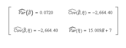
Note that Nelson expresses the results as multiples of 1,000 (or = 26.297, etc.). The published results were adjusted by this factor to correlate with Weibull++ results.
Computed Results in Weibull++
This same data set can be entered into a Weibull++ standard folio, using 2-parameter Weibull and MLE to calculate the parameter estimates.
You can also enter the data as given in table without grouping them by opening a data sheet configured for suspension data. Then click the Group Data icon and chose Group exactly identical values.
The data will be automatically grouped and put into a new grouped data sheet.
Weibull++ computed parameters for maximum likelihood are:
- [math]\displaystyle{ \begin{align}
& \widehat{\beta }=1.0584 \\
& \widehat{\eta} = 26,297 \\
\end{align}\,\! }[/math]
Weibull++ computed 95% FM confidence limits on the parameters:
- [math]\displaystyle{ \begin{align}
& \widehat{\beta }=\lbrace 0.6441, \text{ }1.7394\rbrace \\
& \widehat{\eta} = \lbrace 10,522, \text{ }65,532\rbrace \\
\end{align}\,\! }[/math]
Weibull++ computed/variance covariance matrix:
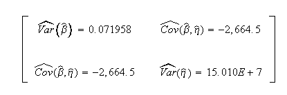
The two-sided 95% bounds on the parameters can be determined from the QCP. Calculate and then click Report to see the results.
Interval Data MLE Example
From Wayne Nelson, Applied Life Data Analysis, Page 415 [30]. 167 identical parts were inspected for cracks. The following is a table of their last inspection times and times-to-failure:
Published Results:
Published results (using MLE):
- [math]\displaystyle{ \begin{align}
& \widehat{\beta }=1.486 \\
& \widehat{\eta} = 71.687\\
\end{align}\,\! }[/math]
Published 95% FM confidence limits on the parameters:
- [math]\displaystyle{ \begin{align}
& \widehat{\beta }=\lbrace 1.224, \text{ }1.802\rbrace \\
& \widehat{\eta} = \lbrace 61.962, \text{ }82.938\rbrace \\
\end{align}\,\! }[/math]
Published variance/covariance matrix:
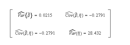
Computed Results in Weibull++
This same data set can be entered into a Weibull++ standard folio that's configured for grouped times-to-failure data with suspensions and interval data.
Weibull++ computed parameters for maximum likelihood are:
- [math]\displaystyle{ \begin{align}
& \widehat{\beta }=1.485 \\
& \widehat{\eta} = 71.690\\
\end{align}\,\! }[/math]
Weibull++ computed 95% FM confidence limits on the parameters:
- [math]\displaystyle{ \begin{align}
& \widehat{\beta }=\lbrace 1.224, \text{ }1.802\rbrace \\
& \widehat{\eta} = \lbrace 61.961, \text{ }82.947\rbrace \\
\end{align}\,\! }[/math]
Weibull++ computed/variance covariance matrix:
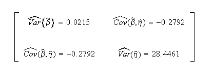
Grouped Suspension MLE Example
From Dallas R. Wingo, IEEE Transactions on Reliability Vol. R-22, No 2, June 1973, Pages 96-100.
Wingo uses the following times-to-failure: 37, 55, 64, 72, 74, 87, 88, 89, 91, 92, 94, 95, 97, 98, 100, 101, 102, 102, 105, 105, 107, 113, 117, 120, 120, 120, 122, 124, 126, 130, 135, 138, 182. In addition, the following suspensions are used: 4 at 70, 5 at 80, 4 at 99, 3 at 121 and 1 at 150.
Published Results (using MLE)
- [math]\displaystyle{ \begin{align}
& \widehat{\beta }=3.7596935\\
& \widehat{\eta} = 106.49758 \\
& \hat{\gamma }=14.451684\\
\end{align}\,\! }[/math]
Computed Results in Weibull++
- [math]\displaystyle{ \begin{align}
& \widehat{\beta }=3.7596935\\
& \widehat{\eta} = 106.49758 \\
& \hat{\gamma }=14.451684\\
\end{align}\,\! }[/math]
Note that you must select the Use True 3-P MLEoption in the Weibull++ Application Setup to replicate these results.
3-P Probability Plot Example
Suppose we want to model a left censored, right censored, interval, and complete data set, consisting of 274 units under test of which 185 units fail. The following table contains the data.
The Test Data
| Data Point Index
|
Number in State
|
Last Inspection
|
State (S or F)
|
State End Time
|
| 1 |
2 |
5 |
F |
5
|
| 2 |
23 |
5 |
S |
5
|
| 3 |
28 |
0 |
F |
7
|
| 4 |
4 |
10 |
F |
10
|
| 5 |
7 |
15 |
F |
15
|
| 6 |
8 |
20 |
F |
20
|
| 7 |
29 |
20 |
S |
20
|
| 8 |
32 |
0 |
F |
22
|
| 9 |
6 |
25 |
F |
25
|
| 10 |
4 |
27 |
F |
30
|
| 11 |
8 |
30 |
F |
35
|
| 12 |
5 |
30 |
F |
40
|
| 13 |
9 |
27 |
F |
45
|
| 14 |
7 |
25 |
F |
50
|
| 15 |
5 |
20 |
F |
55
|
| 16 |
3 |
15 |
F |
60
|
| 17 |
6 |
10 |
F |
65
|
| 18 |
3 |
5 |
F |
70
|
| 19 |
37 |
100 |
S |
100
|
| 20 |
48 |
0 |
F |
102
|
Solution
Since standard ranking methods for dealing with these different data types are inadequate, we will want to use the ReliaSoft ranking method. This option is the default in Weibull++ when dealing with interval data. The filled-out standard folio is shown next:
The computed parameters using MLE are:
- [math]\displaystyle{ \hat{\beta }=0.748;\text{ }\hat{\eta }=44.38\,\! }[/math]
Using RRX:
- [math]\displaystyle{ \hat{\beta }=1.057;\text{ }\hat{\eta }=36.29\,\! }[/math]
Using RRY:
- [math]\displaystyle{ \hat{\beta }=0.998;\text{ }\hat{\eta }=37.16\,\! }[/math]
The plot with the two-sided 90% confidence bounds for the rank regression on X solution is:


![Effect on [math]\displaystyle{ \beta\,\! }[/math] on the cdf on the Weibull probability plot with a fixed value of [math]\displaystyle{ \eta\,\! }[/math]](/index.php/File:WB.8_effect_of_weibull.png)
![The effect of values of [math]\displaystyle{ \beta\,\! }[/math] on the Weibull reliability plot.](/index.php/File:WB.8_weibull_reliability.png)
![The effect of [math]\displaystyle{ \beta\,\! }[/math] on the Weibull failure rate function.](/index.php/File:WB.8_weibull_failure.png)
![The effects of [math]\displaystyle{ \eta\,\! }[/math] on the Weibull pdf for a common [math]\displaystyle{ \beta\,\! }[/math].](/index.php/File:WB.8_effects_of_n.png)
![The effect of a positive location parameter, [math]\displaystyle{ \gamma\,\! }[/math], on the position of the Weibull pdf.](/index.php/File:WB.8_location_parameter.png)


