Template:Example: Weibull Distribution Interval Data Example: Difference between revisions
Jump to navigation
Jump to search
No edit summary |
No edit summary |
||
| Line 41: | Line 41: | ||
The computed parameters using maximum likelihood are: | The computed parameters using maximum likelihood are: | ||
::<math>\begin{align} | |||
& \hat{\beta }=5.76 \\ | & \hat{\beta }=5.76 \\ | ||
& \hat{\eta }=44.68 \\ | & \hat{\eta }=44.68 \\ | ||
\end{align}</math | \end{align}</math> | ||
using RRX or rank regression on X: | using RRX or rank regression on X: | ||
::<math>\begin{align} | |||
& \hat{\beta }=5.70 \\ | & \hat{\beta }=5.70 \\ | ||
& \hat{\eta }=44.54 \\ | & \hat{\eta }=44.54 \\ | ||
\end{align}</math | \end{align}</math> | ||
and using RRY or rank regression on Y: | and using RRY or rank regression on Y: | ||
::<math>\begin{align} | |||
& \hat{\beta }=5.41 \\ | & \hat{\beta }=5.41 \\ | ||
& \hat{\eta }=44.76 \\ | & \hat{\eta }=44.76 \\ | ||
\end{align}</math | \end{align}</math> | ||
The plot of the MLE solution with the two-sided 90% confidence bounds is: | The plot of the MLE solution with the two-sided 90% confidence bounds is: | ||
[[Image: MLE Plot.png|center|550px]] | [[Image: MLE Plot.png|center|550px]] | ||
Revision as of 05:27, 6 August 2012
Weibull Distribution Interval Data Example
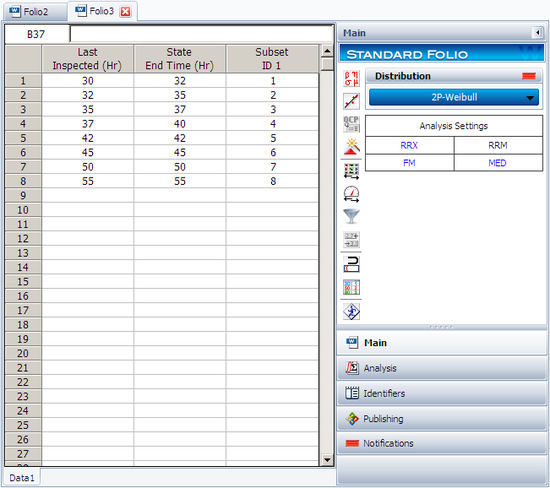
Suppose that we have run an experiment with eight units being tested and the following is a table of their last inspection times and times-to-failure:
| Data Point Index | Last Inspection | Time to Failure |
| 1 | 30 | 32 |
| 2 | 32 | 35 |
| 3 | 35 | 37 |
| 4 | 37 | 40 |
| 5 | 42 | 42 |
| 6 | 45 | 45 |
| 7 | 50 | 50 |
| 8 | 55 | 55 |
Analyze the data using several different parameter estimation techniques and compare the results.
Solution
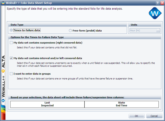
This data set can be entered into Weibull++ by opening a new Data Folio and choosing Times-to-failure and My data set contains interval and/or left censored data.

The data is entered as follows,

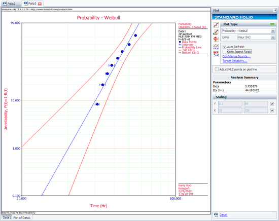
The computed parameters using maximum likelihood are:
- [math]\displaystyle{ \begin{align} & \hat{\beta }=5.76 \\ & \hat{\eta }=44.68 \\ \end{align} }[/math]
using RRX or rank regression on X:
- [math]\displaystyle{ \begin{align} & \hat{\beta }=5.70 \\ & \hat{\eta }=44.54 \\ \end{align} }[/math]
and using RRY or rank regression on Y:
- [math]\displaystyle{ \begin{align} & \hat{\beta }=5.41 \\ & \hat{\eta }=44.76 \\ \end{align} }[/math]
The plot of the MLE solution with the two-sided 90% confidence bounds is:
