Template:Estimation of the Weibull Parameters
Estimation of the Weibull Parameters
The estimates of the parameters of the Weibull distribution can be found graphically via probability plotting paper, or analytically, either using least squares or maximum likelihood.
Probability Plotting
One method of calculating the parameters of the Weibull distribution is by using probability plotting. To better illustrate this procedure, consider the following example from Kececioglu [20].
Example 1
Assume that six identical units are being reliability tested at the same application and operation stress levels. All of these units fail during the test after operating the following number of hours, Ti: 93, 34, 16, 120, 53 and 75. Estimate the values of the parameters for a two-parameter Weibull distribution and determine the reliability of the units at a time of 15 hours.
Solution to Example 1
The steps for determining the parameters of the Weibull representing the data, using probability plotting, are outlined in the following instructions. First, rank the times-to-failure in ascending order as shown next.
| Time-to-failure, hrs |
Failure Order Number out of Sample Size of 6 |
|---|---|
| 16 | 1 |
| 34 | 2 |
| 53 | 3 |
| 75 | 4 |
| 93 | 5 |
| 120 | 6 |
Obtain their median rank plotting positions. Median rank positions are used instead of other ranking methods because median ranks are at a specific confidence level (50%). Median ranks can be found tabulated in many reliability books. They can also be estimated using the following equation,
- [math]\displaystyle{ MR \sim { \frac{i-0.3}{N+0.4}}\cdot 100, }[/math]
where [math]\displaystyle{ i }[/math] is the failure order number and [math]\displaystyle{ N }[/math] is the total sample size. The exact median ranks are found in Weibull++ by solving,
- [math]\displaystyle{ \sum_{k=i}^N{\binom{N}{k}}{MR^k}{(1-MR)^{N-k}}=0.5=50% }[/math]
for [math]\displaystyle{ MR }[/math], where [math]\displaystyle{ N }[/math] is the sample size and [math]\displaystyle{ i }[/math] the order number. The times-to-failure, with their corresponding median ranks, are shown next.
| Time-to-failure, hrs | Median Rank,% |
|---|---|
| 16 | 10.91 |
| 34 | 26.44 |
| 53 | 42.14 |
| 75 | 57.86 |
| 93 | 73.56 |
| 120 | 89.1 |
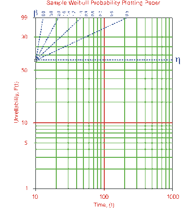
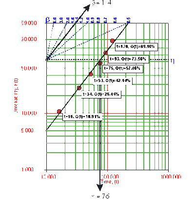
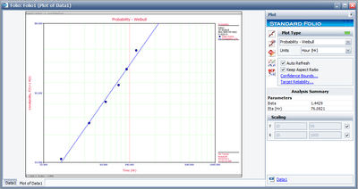
On a Weibull probability paper, plot the times and their corresponding ranks. A sample of a Weibull probability paper is given in Figure 6-7 and the plot of the data in the example in Figure 6-8.
Draw the best possible straight line through these points, as shown below, then obtain the slope of this line by drawing a line, parallel to the one just obtained, through the slope indicator. This value is the estimate of the shape parameter [math]\displaystyle{ \hat{\beta } }[/math], in this case [math]\displaystyle{ \hat{\beta }=1.4 }[/math].
At the [math]\displaystyle{ Q(t)=63.2% }[/math] ordinate point, draw a straight horizontal line until this line intersects the fitted straight line. Draw a vertical line through this intersection until it crosses the abscissa. The value at the intersection of the abscissa is the estimate of [math]\displaystyle{ \hat{\eta } }[/math]. For this case, [math]\displaystyle{ \hat{\eta }=76 }[/math] hours. (This is always at 63.2% since: [math]\displaystyle{ Q(T)=1-e^{-(\frac{\eta }{\eta })^{\beta }}=1-e^{-1}=0.632=63.2% }[/math].
Now any reliability value for any mission time [math]\displaystyle{ t }[/math] can be obtained. For example, the reliability for a mission of 15 hours, or any other time, can now be obtained either from the plot or analytically. To obtain the value from the plot, draw a vertical line from the abscissa, at hours, to the fitted line. Draw a horizontal line from this intersection to the ordinate and read Q(t), in this case [math]\displaystyle{ Q(t)=9.8% }[/math]. Thus, [math]\displaystyle{ R(t)=1-Q(t)=90.2% }[/math]. This can also be obtained analytically from the Weibull reliability function since the estimates of both of the parameters are known or:
[math]\displaystyle{ R(t=15)=e^{-\left( \frac{15}{\eta }\right) ^{\beta }}=e^{-\left( \frac{15}{76 }\right) ^{1.4}}=90.2% }[/math]
Probability Plotting for the Location Parameter, γ
The third parameter of the Weibull distribution is utilized when the data do not fall on a straight line, but fall on either a concave up or down curve. The following statements can be made regarding the value of γ:
- Case 1: If the curve for MR versus Tj is concave down and the curve for MR versus (Tj − T1) is concave up, then there exists a γ such that 0 < γ < T1, or γ has a positive value.
- Case 2: If the curves for MR versus Tj and MR versus (Tj − T1) are both concave up, then there exists a negative γ which will straighten out the curve of MR versus Tj.
- Case 3: If neither one of the previous two cases prevails, then either reject the Weibull as one capable of representing the data, or proceed with the multiple population (mixed Weibull) analysis. To obtain the location parameter, γ:
- Subtract the same arbitrary value, γ, from all the times to failure and replot the data.
- If the initial curve is concave up, subtract a negative γ from each failure time.
- If the initial curve is concave down, subtract a positive γ from each failure time.
- Repeat until the data plots on an acceptable straight line.
- The value of γ is the subtracted (positive or negative) value that places the points in an acceptable straight line.
The other two parameters are then obtained using the techniques previously described. Also, it is important to note that we used the term subtract a positive or negative gamma, where subtracting a negative gamma is equivalent to adding it. Note that when adjusting for gamma, the x-axis scale for the straight line becomes (T − γ).
Example 2
Six identical units are reliability tested under the same stresses and conditions. All units are tested to failure and the following times-to-failure are recorded: 48, 66, 85, 107, 125 and 152 hours. Find the parameters of the three-parameter Weibull distribution using probability plotting.
Solution to Example 2
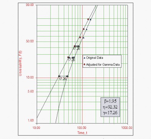
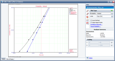
The following figure shows the results. Note that since the original data set was concave down, 17.26 was subtracted from all the times-to-failure and replotted, resulting in a straight line, thus γ = 17.26. (We used Weibull++ to get the results. To perform this by hand, one would attempt different values of γ, using a trial and error methodology, until an acceptable straight line is found. When performed manually, you do not expect decimal accuracy.)
Rank Regression on Y
Performing rank regression on Y requires that a straight line mathematically be fitted to a set of data points such that the sum of the squares of the vertical deviations from the points to the line is minimized. This is in essence the same methodology as the probability plotting method, except that we use the principle of least squares to determine the line through the points, as opposed to just eyeballing it. The first step is to bring our function into a linear form. For the two-parameter Weibull distribution, the (cumulative density function) is:
- [math]\displaystyle{ F(T)=1-e^{-\left( \frac{T}{\eta }\right) ^{\beta }} (Fw) }[/math]
Taking the natural logarithm of both sides of the equation yields:
- [math]\displaystyle{ \ln[ 1-F(T)] =-( \frac{T}{\eta }) ^{\beta } }[/math]
- [math]\displaystyle{ \ln{ -\ln[ 1-F(T)]} =\beta \ln ( \frac{T}{ \eta }) }[/math]
- or:
- [math]\displaystyle{ \ln \{ -\ln[ 1-F(T)]\} =-\beta \ln (\eta )+\beta \ln (T) EQNREF logw }[/math]
- Now let:
- [math]\displaystyle{ y = \ln \{ -\ln[ 1-F(T)]\} ( yw ) }[/math]
- [math]\displaystyle{ a = − βln(\eta) }[/math] (aw)
- and:
- [math]\displaystyle{ b= \beta }[/math] ( bw )
which results in the linear equation of:
- [math]\displaystyle{ y=a+bx }[/math]
The least squares parameter estimation method (also known as regression analysis) was discussed in Chapter 3 and the following equations for regression on Y were derived in Appendix A:
- [math]\displaystyle{ \hat{a}=\frac{\sum\limits_{i=1}^{N}y_{i}}{N}-\hat{b}\frac{ \sum\limits_{i=1}^{N}x_{i}}{N}=\bar{y}-\hat{b}\bar{x} EQNREF aaw }[/math]
- and:
- [math]\displaystyle{ \hat{b}={\frac{\sum\limits_{i=1}^{N}x_{i}y_{i}-\frac{\sum \limits_{i=1}^{N}x_{i}\sum\limits_{i=1}^{N}y_{i}}{N}}{\sum \limits_{i=1}^{N}x_{i}^{2}-\frac{\left( \sum\limits_{i=1}^{N}x_{i}\right) ^{2}}{N}}} EQNREF bbw }[/math]
In this case the equations for yi and xi are:
- [math]\displaystyle{ y_{i}=\ln \left\{ -\ln [1-F(T_{i})]\right\} , }[/math]
- and:
- xi = ln(Ti).
The [math]\displaystyle{ F(T_{i})^{\prime }s }[/math] are estimated from the median ranks.
Once [math]\displaystyle{ \hat{a} }[/math] and [math]\displaystyle{ \hat{b} }[/math] are obtained, then [math]\displaystyle{ \hat{\beta } }[/math] and [math]\displaystyle{ \hat{\eta } }[/math] can easily be obtained from Eqns. (EQNREF aw ) and (\ref {bw}).
The Correlation Coefficient
The correlation coefficient is defined as follows:
- [math]\displaystyle{ \rho ={\frac{\sigma _{xy}}{\sigma _{x}\sigma _{y}}} }[/math]
where, σx y = covariance of and , σx = standard deviation of , and σy = standard deviation of . The estimator of ρ is the sample correlation coefficient, [math]\displaystyle{ \hat{\rho} }[/math], given by:
- [math]\displaystyle{ \hat{\rho}=\frac{\sum\limits_{i=1}^{N}(x_{i}-\overline{x})(y_{i}-\overline{y} )}{\sqrt{\sum\limits_{i=1}^{N}(x_{i}-\overline{x})^{2}\cdot \sum\limits_{i=1}^{N}(y_{i}-\overline{y})^{2}}} EQNREF RHOw }[/math]
Example 3
Consider the data in Example 1, where six units were tested to failure and the following failure times were recorded: 16, 34, 53, 75, 93 and 120 hours. Estimate the parameters and the correlation coefficient using rank regression on Y, assuming that the data follow the two-parameter Weibull distribution.
Solution to Example 3
Construct a table as shown below.
| Table 6.1 - Least Squares Analysis | |||||||
| [math]\displaystyle{ N }[/math] | [math]\displaystyle{ T_{i} }[/math] | [math]\displaystyle{ ln(T_{i}) }[/math] | [math]\displaystyle{ F(T_i) }[/math] | [math]\displaystyle{ y_{i} }[/math] | [math]\displaystyle{ (ln{T_i})^2 }[/math] | [math]\displaystyle{ {y_i}^2 }[/math] | [math]\displaystyle{ (ln{T_i})y_i }[/math] |
|---|---|---|---|---|---|---|---|
| 1 | 16 | 2.7726 | 0.1091 | -2.1583 | 7.6873 | 4.6582 | -5.9840 |
| 2 | 34 | 3.5264 | 0.2645 | -1.1802 | 12.4352 | 1.393 | -4.1620 |
| 3 | 53 | 3.9703 | 0.4214 | -0.6030 | 15.7632 | 0.3637 | -2.3943 |
| 4 | 75 | 4.3175 | 0.5786 | -0.146 | 18.6407 | 0.0213 | -0.6303 |
| 5 | 93 | 4.5326 | 0.7355 | 0.2851 | 20.5445 | 0.0813 | 1.2923 |
| 6 | 120 | 4.7875 | 0.8909 | 0.7955 | 22.9201 | 0.6328 | 3.8083 |
| [math]\displaystyle{ \sum }[/math] | 23.9068 | -3.007 | 97.9909 | 7.1502 | -8.0699 | ||
Utilizing the values from Table 6.1, calculate [math]\displaystyle{ \hat{a} }[/math] and [math]\displaystyle{ \hat{b} }[/math] using Eqns. (EQNREF aaw ) and (EQNREF bbw ):
- [math]\displaystyle{ \hat{b} =\frac{\sum\limits_{i=1}^{6}(\ln T_{i})y_{i}-(\sum\limits_{i=1}^{6}\ln T_{i})(\sum\limits_{i=1}^{6}y_{i})/6}{ \sum\limits_{i=1}^{6}(\ln T_{i})^{2}-(\sum\limits_{i=1}^{6}\ln T_{i})^{2}/6} }[/math]
- [math]\displaystyle{ \hat{b}=\frac{-8.0699-(23.9068)(-3.0070)/6}{97.9909-(23.9068)^{2}/6} }[/math]
- or
- [math]\displaystyle{ \hat{b}=1.4301 }[/math]
- and:
- [math]\displaystyle{ \hat{a}=\overline{y}-\hat{b}\overline{T}=\frac{\sum \limits_{i=1}^{N}y_{i}}{N}-\hat{b}\frac{\sum\limits_{i=1}^{N}\ln T_{i}}{N } }[/math]
- or:
- [math]\displaystyle{ \hat{a}=\frac{(-3.0070)}{6}-(1.4301)\frac{23.9068}{6}=-6.19935 }[/math]
Therefore, from Eqn. (EQNREF bw ):
- [math]\displaystyle{ \hat{\beta }=\hat{b}=1.4301 }[/math]
and from Eqn. (EQNREF aw ):
- [math]\displaystyle{ \hat{\eta }=e^{-\frac{\hat{a}}{\hat{b}}}=e^{-\frac{(-6.19935)}{ 1.4301}} }[/math]
- or:
- [math]\displaystyle{ \hat{\eta }=76.318\text{ hr} }[/math]
The correlation coefficient can be estimated using Eqn. (EQNREF RHOw ):
- [math]\displaystyle{ \hat{\rho }=0.9956 }[/math]
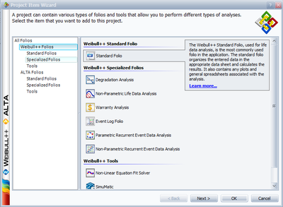
The above example can be repeated using Weibull++. Start Weibull++ and create a new Data Folio.
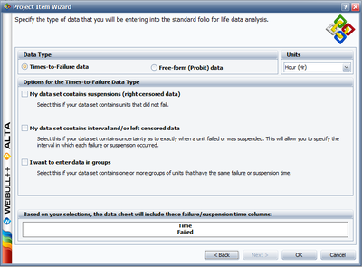
Select the Times-to-failure data option.
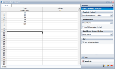
Enter the times-to-failure in the datasheet (ignore the Subset ID column), as shown next. The times-to-failure need not be sorted, Weibull++ will automatically sort the data.
Select the desired method of analysis. Note that we are assuming that the underlying distribution is the Weibull, so make sure that the Weibull distribution is selected. Under Parameters/Type on the Main page, select 2.
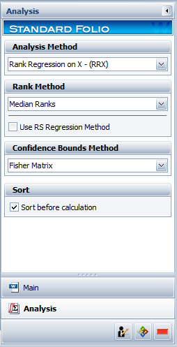
Also, so that you get the same results as this example, switch to the Analysis page and make sure you are using the Rank Regression on Y (RRY) calculation method with this example, as shown next.
Note that this can also be done from the Main page by clicking the left bottom box under the Results area. Each time you click that box you will see the method switch between MLE, RRX, and RRY. Click the Calculate icon,
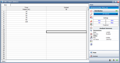
or select Calculate from the Data menu. The results will appear in the Data Folio's Results area. The next figure shows the results for this example.
You can now plot the results by clicking the Plot icon,
or by selecting Plot Probability from the Data menu.
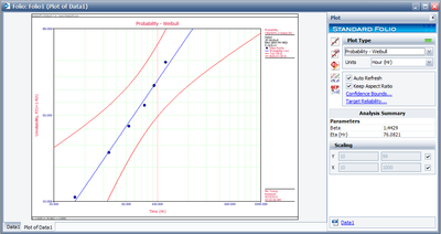
The Weibull probability plot for these data is shown next.
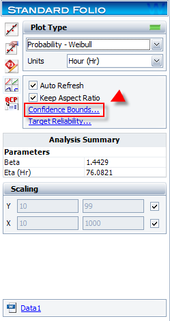
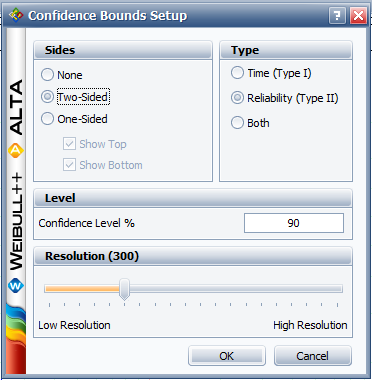
The confidence bounds, as determined from the Fisher matrix, can also be plotted. Select Confidence Bounds from the Plot menu, choose Two-Sided under Sides, Reliability (Type II) under Type and enter 90 for the Confidence level.
The plot will appear as follows,
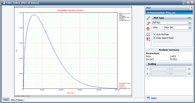
If desired, the Weibull [math]\displaystyle{ pdf }[/math] representing these data can be written as:
- [math]\displaystyle{ f(T)={\frac{\beta }{\eta }}\left( {\frac{T}{\eta }}\right) ^{\beta -1}e^{-\left( {\frac{T}{\eta }}\right) ^{\beta }} }[/math]
- or:
- [math]\displaystyle{ f(T)={\frac{1.4302}{76.317}}\left( {\frac{T}{76.317}}\right) ^{0.4302}e^{-\left( {\frac{T}{76.317}}\right) ^{1.4302}} }[/math] You can also plot the Weibull by selecting Pdf Plot from the Plot Type drop-down menu on the control panel to the right of the plot area.
From this point on, different results, reports and plots can be obtained.
Rank Regression on X
Performing a rank regression on X is similar to the process for rank regression on Y, with the difference being that the horizontal deviations from the points to the line are minimized rather than the vertical. Again, the first task is to bring our function, Eqn. (EQNREF Fw ), into a linear form. This step is exactly the same as in the regression on Y analysis and Eqns. (EQNREF logw ), (EQNREF yw ), (EQNREF aw ) and (EQNREF bw ) apply in this case too. The derivation from the previous analysis begins on the least squares fit part, where in this case we treat as the dependent variable and as the independent variable. The best-fitting straight line to the data, for regression on X (see Chapter 3), is the straight line:
- [math]\displaystyle{ x= \hat{a}+\hat{b}y }[/math] EQNREF xlinew
The corresponding equations for [math]\displaystyle{ \hat{a} }[/math] and [math]\displaystyle{ \hat{b} }[/math] are:
- [math]\displaystyle{ \hat{a}=\overline{x}-\hat{b}\overline{y}=\frac{\sum\limits_{i=1}^{N}x_{i}}{N} -\hat{b}\frac{\sum\limits_{i=1}^{N}y_{i}}{N} }[/math]
- and
- [math]\displaystyle{ \hat{b}={\frac{\sum\limits_{i=1}^{N}x_{i}y_{i}-\frac{\sum \limits_{i=1}^{N}x_{i}\sum\limits_{i=1}^{N}y_{i}}{N}}{\sum \limits_{i=1}^{N}y_{i}^{2}-\frac{\left( \sum\limits_{i=1}^{N}y_{i}\right) ^{2}}{N}}} }[/math]
- where:
- [math]\displaystyle{ y_{i}=\ln \left\{ -\ln [1-F(T_{i})]\right\} }[/math] and:
xi = ln(Ti) and the F(Ti) values are again obtained from the median ranks.
Once [math]\displaystyle{ \hat{a} }[/math] and [math]\displaystyle{ \hat{b} }[/math] are obtained, solve Eqn. (EQNREF xlinew ) for y, which corresponds to:
- [math]\displaystyle{ y=-\frac{\hat{a}}{\hat{b}}+\frac{1}{\hat{b}}x }[/math] Solving for the parameters from Eqns. (EQNREF aw ) and (EQNREF bw ) we get
- [math]\displaystyle{ a=-\frac{\hat{a}}{\hat{b}}=-\beta \ln (\eta ) }[/math] EQNREF awx
- and
- [math]\displaystyle{ b=\frac{1}{\hat{b}}=\beta EQNREF bwx }[/math] The correlation coefficient is evaluated as before using Eqn. (EQNREF RHOw ).
Example 4
Repeat Example 1 using rank regression on X.
Solution to Example 4
Solution to Example 4 Table 6.1, constructed in Example 3, can also be applied to this example.
Using the values from this table we get:
- [math]\displaystyle{ \hat{b} ={\frac{\sum\limits_{i=1}^{6}(\ln T_{i})y_{i}-\frac{ \sum\limits_{i=1}^{6}\ln T_{i}\sum\limits_{i=1}^{6}y_{i}}{6}}{ \sum\limits_{i=1}^{6}y_{i}^{2}-\frac{\left( \sum\limits_{i=1}^{6}y_{i}\right) ^{2}}{6}}} }[/math]
- [math]\displaystyle{ \hat{b} =\frac{-8.0699-(23.9068)(-3.0070)/6}{7.1502-(-3.0070)^{2}/6} }[/math]
- or:
- [math]\displaystyle{ \hat{b}=0.6931 }[/math]
- and:
- [math]\displaystyle{ \hat{a}=\overline{x}-\hat{b}\overline{y}=\frac{\sum\limits_{i=1}^{6}\ln T_{i} }{6}-\hat{b}\frac{\sum\limits_{i=1}^{6}y_{i}}{6} }[/math]
- or:
- [math]\displaystyle{ \hat{a}=\frac{23.9068}{6}-(0.6931)\frac{(-3.0070)}{6}=4.3318 }[/math]
Therefore, from Eqn. (EQNREF bwx ):
- [math]\displaystyle{ \hat{\beta }=\frac{1}{\hat{b}}=\frac{1}{0.6931}=1.4428 }[/math]
- and from Eqn. (EQNREF awx )
- [math]\displaystyle{ \hat{\eta }=e^{\frac{\hat{a}}{\hat{b}}\cdot \frac{1}{\hat{ \beta }}}=e^{\frac{4.3318}{0.6931}\cdot \frac{1}{1.4428}}=76.0811\text{ hr} }[/math]
The correlation coefficient is found using Eqn. (EQNREF RHOw ):
- [math]\displaystyle{ \hat{\rho }=0.9956 }[/math]
The results and the associated graph using Weibull++ are given next. Note that the slight variation in the results is due to the number of significant figures used in the estimation of the median ranks. Weibull++ by default uses double precision accuracy when computing the median ranks.
Three-Parameter Weibull Regression
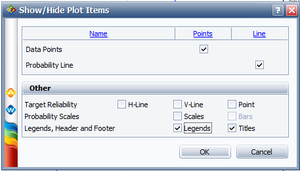
When the MR versus Tj points plotted on the Weibull probability paper do not fall on a satisfactory straight line and the points fall on a curve,(Note that other shapes, particularly shapes, might suggest the existence of more than one population. In these cases, the multiple population, mixed Weibull distribution, may be more appropriate. Chapter 10 presents the mixed Weibull distribution.) then a location parameter, γ, might exist which may straighten out these points. The goal in this case is to fit a curve, instead of a line, through the data points using nonlinear regression. The Gauss-Newton method can be used to solve for the parameters, β, η and γ, by performing a Taylor series expansion on F(Ti;β,η,γ). Then the nonlinear model is approximated with linear terms and ordinary least squares are employed to estimate the parameters. This procedure is iterated until a satisfactory solution is reached. Weibull++ 7 calculates the value of γ by utilizing an optimized Nelder-Mead algorithm, and adjusts the points by this value of γ such that they fall on a straight line, and then plots both the adjusted and the original unadjusted points. To draw a curve through the original unadjusted points, if so desired, select Weibull 3P Line Unadjusted for Gamma from the Show Plot Line submenu under the Plot Options menu. The returned estimations of the parameters are the same when selecting RRX or RRY. To display the unadjusted data points and line along with the adjusted data points and line, select Show/Hide Items under the Plot Options menu and include the unadjusted data points and line as follows:
The results and the associated graph for the previous example using the three-parameter Weibull case are shown next:
Maximum Likelihood Estimation
As outlined in Chapter 3, maximum likelihood estimation works by developing a likelihood function based on the available data and finding the values of the parameter estimates that maximize the likelihood function. This can be achieved by using iterative methods to determine the parameter estimate values that maximize the likelihood function, but this can be rather difficult and time-consuming, particularly when dealing with the three-parameter distribution. Another method of finding the parameter estimates involves taking the partial derivatives of the likelihood function with respect to the parameters, setting the resulting equations equal to zero and solving simultaneously to determine the values of the parameter estimates. ( Note that MLE asymptotic properties do not hold when estimating γ using MLE [27].) The log-likelihood functions and associated partial derivatives used to determine maximum likelihood estimates for the Weibull distribution are covered in Appendix C.
Example 5
Repeat Example 1 using maximum likelihood estimation.
Solution to Example 5
In this case, we have non-grouped data with no suspensions or intervals, i.e. complete data. The equations for the partial derivatives of the log-likelihood function are derived in Appendix C and given next:
- [math]\displaystyle{ \frac{\partial \Lambda }{\partial \beta }=\frac{6}{\beta } +\sum_{i=1}^{6}\ln \left( \frac{T_{i}}{\eta }\right) -\sum_{i=1}^{6}\left( \frac{T_{i}}{\eta }\right) ^{\beta }\ln \left( \frac{T_{i}}{\eta }\right) =0 }[/math]
- and:
- [math]\displaystyle{ \frac{\partial \Lambda }{\partial \eta }=\frac{-\beta }{\eta }\cdot 6+\frac{ \beta }{\eta }\sum\limits_{i=1}^{6}\left( \frac{T_{i}}{\eta }\right) ^{\beta }=0 }[/math]
Solving the above equations simultaneously we get:
- [math]\displaystyle{ \hat{\beta }=1.933, }[/math] [math]\displaystyle{ \hat{\eta }=73.526 }[/math]
The variance/covariance matrix is found to be,
- [math]\displaystyle{ \left[ \begin{array}{ccc} \hat{Var}\left( \hat{\beta }\right) =0.4211 & \hat{Cov}( \hat{\beta },\hat{\eta })=3.272 \\ \hat{Cov}(\hat{\beta },\hat{\eta })=3.272 & \hat{Var} \left( \hat{\eta }\right) =266.646 \end{array} \right] }[/math]
The results and the associated graph using Weibull++ (MLE) are shown next.
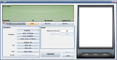
You can view the variance/covariance matrix directly by clicking the Quick Calculation Pad (QCP) icon
Note that the decimal accuracy displayed and used is based on your individual User Setup.
