Target Reliability Tool: Difference between revisions
Lisa Hacker (talk | contribs) No edit summary |
|||
| (41 intermediate revisions by 6 users not shown) | |||
| Line 1: | Line 1: | ||
{{ | {{Template:LDABOOK|Additional Reliability Analysis Tools|Target Reliability Tool}} | ||
Product reliability affects total product costs in multiple ways. Increasing reliability increases the initial cost of production but decreases other costs incurred over the life of the product. For example, increased reliability results in lower warranty and replacement costs for defective products. Increased reliability also results in greater market share because satisfied customers typically become repeat customers and recommend reliable products to others. A minimal total product cost can be determined by calculating the optimum reliability for such a product. The Target Reliability tool in Weibull++ does this by minimizing the sum of lost sales costs, warranty costs and manufacturing costs. | |||
=Cost Factors in Determining Target Reliability= | |||
==Lost Sales Cost== | |||
The lost sales cost is caused due to lost market share. It is caused by customers choosing to go elsewhere for goods and services. The lost sales cost depends on the total market value for a product and the actual sales revenue of a product. | |||
<center><font size="3"> | |||
''Lost Sales Cost'' = ''Max'' {0, ''Total Market Value'' - ''Sales Revenue''} | |||
</font></center> | |||
In Weibull++, we assume the total potential market value is the product of maximum market potential (number of units that could be sold) and the best unit sale price. | |||
<center><font size="3"> | |||
''Total Market Value'' = ''Maximum Market Potential'' x ''Best Market Unit Sale Price'' | |||
</font></center> | |||
For example, if the maximum number of units demanded by the market is 100,000 and the best market unit sale price is $12.00, then the total market value would be: | |||
<center><font size="3"> | |||
''100,000'' x ''$12.00'' = ''$1,200,000.00 | |||
</font></center> | |||
Calculating sales revenue requires knowledge of market share and unit sale price. The function for '''market share''' is given by the equation: | |||
<center><math>{{f}_{Market\_Share}}(R)=1-{{e}^{-{{\left( \frac{R}{a} \right)}^{b}}}}\,\!</math></center> | |||
where ''a'' and ''b'' are parameters fitted to market share data, and ''R'' is the product reliability. | |||
The function for '''unit sale price''' is given by: | |||
<center> | <center> | ||
<math> f_{Sale\_Price}\left(R\right)=b\times e^{a\cdot R} \,\!</math> | |||
</center> | |||
where ''a'' and ''b'' are parameters fitted to data, and ''R'' is the product reliability. | |||
As a function of reliability, ''R'', '''sales revenue''' is then calculated as: | |||
<center><font size="3"> | |||
''Sales Revenue'' (''R'') = ''Maximum Market Potential'' x ''Market Share'' (''R'') x ''Unit Price'' (''R'') | |||
</font></center> | |||
Once the total market value and the sales revenue are obtained, they can then be used to calculate the lost sales cost using the formula given at the beginning of this section. | |||
==Production Cost== | |||
Production cost is a function of total market value, market share and manufacturing cost per unit. The function for '''production cost per unit''' is given by: | |||
<center> <math>f_{Production\_Cost} (R)=b\times e^{\frac{a}{\left(1-R\right)}}\,\!</math> </center> | |||
where ''a'' and ''b'' are parameters fitted to data, and ''R'' is the product reliability. | |||
Using the substitution of variable <math> R'=\frac{1}{1-R} \,\!</math> results in the equation: | |||
< | |||
{ | |||
! | |||
</ | |||
<center> <math> f_{Production\_Cost}\left(R'\right)=b\times e^{a\cdot R'} \,\!</math> </center> | |||
[[ | for which the parameters ''a'' and ''b'' can be determined using simple regression tools such as the functions in the [[Degradation Data Analysis]] in Weibull++. | ||
==Warranty Cost== | |||
Warranty cost is a function of total market value, market share, reliability and cost per failure. The function of '''cost per failure''' is given by: | |||
<center> <math>f_{Failure\_Cost}(R)=b\times e^{a\cdot R}\,\!</math> </center> | |||
where ''a'' and ''b'' are parameters fitted to data. For a given reliability value, ''R'', the '''warranty cost''' is given by: | |||
<center><font size="3"> | |||
''Warranty Cost'' (''R'') = ''Maximum Market Potential'' x ''Market Share'' (''R'') x (1 - ''R'') x ''Cost Per Failure'' (''R'') | |||
</font></center> | |||
</center> | |||
==Unreliability Cost== | |||
The sum of the '''Lost Sales Cost''' and '''Warranty Cost''' is called '''Unreliability Cost'''. | |||
==Total Cost== | |||
For a given reliability, ''R'', the expected '''total cost''' is given by: | |||
<center> | <center><font size="3"> | ||
''Total Cost'' (''R'') = ''Lost Sales Cost'' (''R'') + ''Warranty Cost'' (''R'') + ''Production Cost'' (''R'') = ''Unreliability Cost'' (''R'') + ''Production Cost'' (''R'') | |||
</font></center> | |||
</ | |||
< | |||
The | The production cost is a pre-shipping cost, whereas the warranty and lost sales costs are incurred after a product is shipped. These pre- and post-shipping costs can be seen in the figure below. | ||
[[Image: | [[Image:Chart_totalcost.jpg|center|550px| ]] | ||
The reliability value resulting in the lowest total cost will be the target reliability for the product. | |||
= | =Profit and Return at Target Reliability= | ||
With all of the costs described above, the '''profit at a given reliability''' can be calculated as: | |||
<center><font size="3"> | |||
''Profit'' (''R'') = ''Sales Revenue'' - ''Warranty Cost'' (''R'') - ''Production Cost'' (''R'') | |||
</font></center> | |||
= | ==Traditional ROI== | ||
First, consider that traditional Return On Investment (ROI) is a performance measure used to evaluate the efficiency of an investment, or to compare the efficiency of a number of different investments. In general to calculate ROI, the benefit (return) of an investment is divided by the cost of the investment; and the result is expressed as a percentage or a ratio. The following equation illustrates this. | |||
<center> | |||
<math>ROI=\frac{\text{Gain from Investment - Cost of Investment}}{\text{Cost of Investment}}\,\!</math></center> | |||
In this formula, ''Gains from Investment'' refers to the revenue or proceeds obtained due to the investment of interest. | |||
Return on investment is a very popular metric because of its versatility and simplicity. That is, if an investment does not have a positive ROI, or if there are other opportunities with a higher ROI, then the investment should not be undertaken. Reliability ROI is computed in a similar manner by looking at the investment as the the investment in improving the reliability. | |||
==ReliaSoft's Reliability Return on Investment (R3OI)== | |||
R3OI considers the cost and return due to the product reliability. As we discussed before, high reliability will reduce the unreliability cost, but will increase the sales revenue and production cost. A balanced reliability target should be determined based on all of the costs involved. For a given initial investment value, the R3OI is calculated by: | |||
<center> | |||
<math>R3OI=\frac{\text{Profit(R)-Initial Investment }}{\text{Initial Investment}}\,\!</math> | |||
</center> | |||
== | =The Weibull++ Target Reliability Tool= | ||
The purpose of this tool is to qualitatively explore different options with regards to a target reliability for a component, subsystem or system. All the costs are calculated using the equations given above. | |||
There are five inputs | There are five inputs. Specifically: | ||
<br> | <br> | ||
{| border="1" | {| border="1" align="center" style="border-collapse: collapse;" cellpadding="5" cellspacing="5" | ||
|- | |- | ||
! scope="col" | Input Title | ! scope="col" | Input Title | ||
! scope="col" | Input Value | ! scope="col" | Input Value | ||
|- | |- | ||
| Expected failures/returns per | | Expected failures/returns per period (as % of sales) | ||
| valign="middle" align="center" | <math>Q% \text{ where } 0\le Q\le 100 \,\!</math> | | valign="middle" align="center" | <math>Q% \text{ where } 0\le Q\le 100 \,\!</math> | ||
|- | |- | ||
| | | % of market share you expect to capture | ||
| valign="middle" align="center" | <math>S% \text{ where } 0\le S\le 100 \,\!</math> | | valign="middle" align="center" | <math>S% \text{ where } 0\le S\le 100 \,\!</math> | ||
|- | |- | ||
| Line 158: | Line 146: | ||
| valign="middle" align="center" | <math>C \text{ where } 0< C < P+O \,\!</math> | | valign="middle" align="center" | <math>C \text{ where } 0< C < P+O \,\!</math> | ||
|- | |- | ||
| Other costs per failure | | Other costs per failure (in addition to replacement costs) | ||
| valign="middle" align="center" | <math>O \text{ where } 0< O < C+O \,\!</math> | | valign="middle" align="center" | <math>O \text{ where } 0< O < C+O \,\!</math> | ||
|} | |} | ||
| Line 164: | Line 152: | ||
<br> | <br> | ||
These five inputs are then repeated for three specific cases | These five inputs are then repeated for three specific cases: Best Case, Most Likely and Worst Case. | ||
<!-- NOTE: The \,\! is to keep the formula rendered as PNG instead of HTML. Please don't remove it.--> | |||
<br> | <br> | ||
{| border="1" | {| border="1" align="center" style="border-collapse: collapse;" cellpadding="5" cellspacing="5" | ||
|- | |- | ||
! scope="col" | Input Title | ! scope="col" | Input Title | ||
| Line 175: | Line 165: | ||
! scope="col" | Worst Case | ! scope="col" | Worst Case | ||
|- | |- | ||
| valign="middle" align="left" | Expected failures/returns per | | valign="middle" align="left" | Expected failures/returns per period (as % of sales) | ||
| valign="middle" align="center" | <math>{{Q}_{1}}\,\!</math> | | valign="middle" align="center" | <math>{{Q}_{1}}\,\!</math> | ||
| valign="middle" align="center" | <math>{{Q}_{2}}\,\!</math> | | valign="middle" align="center" | <math>{{Q}_{2}}\,\!</math> | ||
| valign="middle" align="center" | <math>{{Q}_{3}}\,\!</math> | | valign="middle" align="center" | <math>{{Q}_{3}}\,\!</math> | ||
|- | |- | ||
| valign="middle" align="left" | | | valign="middle" align="left" | % of market share you expect to capture | ||
| valign="middle" align="center" | <math>{{S}_{1}}\,\!</math> | | valign="middle" align="center" | <math>{{S}_{1}}\,\!</math> | ||
| valign="middle" align="center" | <math>{{S}_{2}}\,\!</math> | | valign="middle" align="center" | <math>{{S}_{2}}\,\!</math> | ||
| Line 195: | Line 185: | ||
| valign="middle" align="center" | <math>{{C}_{3}}\,\!</math> | | valign="middle" align="center" | <math>{{C}_{3}}\,\!</math> | ||
|- | |- | ||
| valign="middle" align="left" | Other costs per failure | | valign="middle" align="left" | Other costs per failure (in addition to replacement costs) | ||
| valign="middle" align="center" | <math>{{O}_{1}}\,\!</math> | | valign="middle" align="center" | <math>{{O}_{1}}\,\!</math> | ||
| valign="middle" align="center" | <math>{{O}_{2}}\,\!</math> | | valign="middle" align="center" | <math>{{O}_{2}}\,\!</math> | ||
| Line 203: | Line 193: | ||
| | ||
Based on the above inputs | Based on the above inputs, four models are then fitted as functions of reliability, <math>R=(1-Q)\,\!</math>, or: | ||
:: <math>\begin{align} | :: <math>\begin{align} | ||
& | & f_{Market\_Share}(R)=1-{{e}^{-{{\left( \frac{R}{a} \right)}^{b}}}} \\ | ||
& | & f_{Sale\_Price}(R)=b\cdot {{e}^{\left( a\cdot R \right)}} \\ | ||
& | & f_{Production\_Cost}(R)=b\cdot {{e}^{\left( a\cdot \left( \frac{1}{1-R} \right) \right)}} \\ | ||
& | & f_{Failure\_Cost}(R)=b\cdot {{e}^{\left( a\cdot R \right)}} \\ | ||
\end{align} | \end{align} | ||
\,\!</math> | \,\!</math> | ||
| Line 215: | Line 205: | ||
| | ||
An additional variable needed | An additional variable needed is '''maximum market potential''', ''M''. It is defined by users in the following input box: | ||
[[Image: Target Reliability Estimator Market Potential icon.png|center|300px]] | |||
All the related costs are defined as given in the previous section and calculated as a function of reliability. The value giving the lowest total cost is the optimal (target) reliability. | |||
==Example== | |||
{{:Target Reliability Tool Example}} | |||
Latest revision as of 19:12, 15 September 2023
Product reliability affects total product costs in multiple ways. Increasing reliability increases the initial cost of production but decreases other costs incurred over the life of the product. For example, increased reliability results in lower warranty and replacement costs for defective products. Increased reliability also results in greater market share because satisfied customers typically become repeat customers and recommend reliable products to others. A minimal total product cost can be determined by calculating the optimum reliability for such a product. The Target Reliability tool in Weibull++ does this by minimizing the sum of lost sales costs, warranty costs and manufacturing costs.
Cost Factors in Determining Target Reliability
Lost Sales Cost
The lost sales cost is caused due to lost market share. It is caused by customers choosing to go elsewhere for goods and services. The lost sales cost depends on the total market value for a product and the actual sales revenue of a product.
Lost Sales Cost = Max {0, Total Market Value - Sales Revenue}
In Weibull++, we assume the total potential market value is the product of maximum market potential (number of units that could be sold) and the best unit sale price.
Total Market Value = Maximum Market Potential x Best Market Unit Sale Price
For example, if the maximum number of units demanded by the market is 100,000 and the best market unit sale price is $12.00, then the total market value would be:
100,000 x $12.00 = $1,200,000.00
Calculating sales revenue requires knowledge of market share and unit sale price. The function for market share is given by the equation:
where a and b are parameters fitted to market share data, and R is the product reliability.
The function for unit sale price is given by:
[math]\displaystyle{ f_{Sale\_Price}\left(R\right)=b\times e^{a\cdot R} \,\! }[/math]
where a and b are parameters fitted to data, and R is the product reliability.
As a function of reliability, R, sales revenue is then calculated as:
Sales Revenue (R) = Maximum Market Potential x Market Share (R) x Unit Price (R)
Once the total market value and the sales revenue are obtained, they can then be used to calculate the lost sales cost using the formula given at the beginning of this section.
Production Cost
Production cost is a function of total market value, market share and manufacturing cost per unit. The function for production cost per unit is given by:
where a and b are parameters fitted to data, and R is the product reliability.
Using the substitution of variable [math]\displaystyle{ R'=\frac{1}{1-R} \,\! }[/math] results in the equation:
for which the parameters a and b can be determined using simple regression tools such as the functions in the Degradation Data Analysis in Weibull++.
Warranty Cost
Warranty cost is a function of total market value, market share, reliability and cost per failure. The function of cost per failure is given by:
where a and b are parameters fitted to data. For a given reliability value, R, the warranty cost is given by:
Warranty Cost (R) = Maximum Market Potential x Market Share (R) x (1 - R) x Cost Per Failure (R)
Unreliability Cost
The sum of the Lost Sales Cost and Warranty Cost is called Unreliability Cost.
Total Cost
For a given reliability, R, the expected total cost is given by:
Total Cost (R) = Lost Sales Cost (R) + Warranty Cost (R) + Production Cost (R) = Unreliability Cost (R) + Production Cost (R)
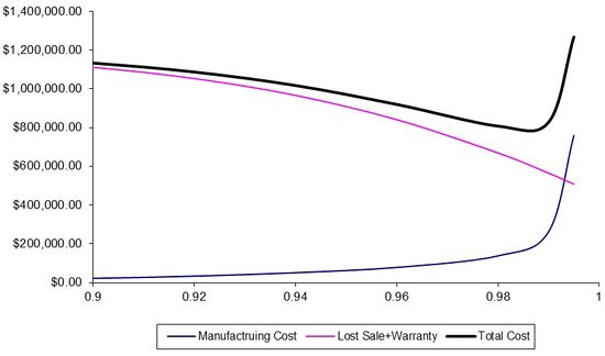
The production cost is a pre-shipping cost, whereas the warranty and lost sales costs are incurred after a product is shipped. These pre- and post-shipping costs can be seen in the figure below.
The reliability value resulting in the lowest total cost will be the target reliability for the product.
Profit and Return at Target Reliability
With all of the costs described above, the profit at a given reliability can be calculated as:
Profit (R) = Sales Revenue - Warranty Cost (R) - Production Cost (R)
Traditional ROI
First, consider that traditional Return On Investment (ROI) is a performance measure used to evaluate the efficiency of an investment, or to compare the efficiency of a number of different investments. In general to calculate ROI, the benefit (return) of an investment is divided by the cost of the investment; and the result is expressed as a percentage or a ratio. The following equation illustrates this.
In this formula, Gains from Investment refers to the revenue or proceeds obtained due to the investment of interest.
Return on investment is a very popular metric because of its versatility and simplicity. That is, if an investment does not have a positive ROI, or if there are other opportunities with a higher ROI, then the investment should not be undertaken. Reliability ROI is computed in a similar manner by looking at the investment as the the investment in improving the reliability.
ReliaSoft's Reliability Return on Investment (R3OI)
R3OI considers the cost and return due to the product reliability. As we discussed before, high reliability will reduce the unreliability cost, but will increase the sales revenue and production cost. A balanced reliability target should be determined based on all of the costs involved. For a given initial investment value, the R3OI is calculated by:
[math]\displaystyle{ R3OI=\frac{\text{Profit(R)-Initial Investment }}{\text{Initial Investment}}\,\! }[/math]
The Weibull++ Target Reliability Tool
The purpose of this tool is to qualitatively explore different options with regards to a target reliability for a component, subsystem or system. All the costs are calculated using the equations given above.
There are five inputs. Specifically:
| Input Title | Input Value |
|---|---|
| Expected failures/returns per period (as % of sales) | [math]\displaystyle{ Q% \text{ where } 0\le Q\le 100 \,\! }[/math] |
| % of market share you expect to capture | [math]\displaystyle{ S% \text{ where } 0\le S\le 100 \,\! }[/math] |
| Average unit sales price | [math]\displaystyle{ P \text{ where } 0\lt P \,\! }[/math] |
| Average cost per unit to produce | [math]\displaystyle{ C \text{ where } 0\lt C \lt P+O \,\! }[/math] |
| Other costs per failure (in addition to replacement costs) | [math]\displaystyle{ O \text{ where } 0\lt O \lt C+O \,\! }[/math] |
These five inputs are then repeated for three specific cases: Best Case, Most Likely and Worst Case.
| Input Title | Best Case | Most Likely | Worst Case |
|---|---|---|---|
| Expected failures/returns per period (as % of sales) | [math]\displaystyle{ {{Q}_{1}}\,\! }[/math] | [math]\displaystyle{ {{Q}_{2}}\,\! }[/math] | [math]\displaystyle{ {{Q}_{3}}\,\! }[/math] |
| % of market share you expect to capture | [math]\displaystyle{ {{S}_{1}}\,\! }[/math] | [math]\displaystyle{ {{S}_{2}}\,\! }[/math] | [math]\displaystyle{ {{S}_{3}}\,\! }[/math] |
| Average unit sales price | [math]\displaystyle{ {{P}_{1}}\,\! }[/math] | [math]\displaystyle{ {{P}_{2}}\,\! }[/math] | [math]\displaystyle{ {{P}_{3}}\,\! }[/math] |
| Average cost per unit to produce | [math]\displaystyle{ {{C}_{1}}\,\! }[/math] | [math]\displaystyle{ {{C}_{2}}\,\! }[/math] | [math]\displaystyle{ {{C}_{3}}\,\! }[/math] |
| Other costs per failure (in addition to replacement costs) | [math]\displaystyle{ {{O}_{1}}\,\! }[/math] | [math]\displaystyle{ {{O}_{2}}\,\! }[/math] | [math]\displaystyle{ {{O}_{3}}\,\! }[/math] |
Based on the above inputs, four models are then fitted as functions of reliability, [math]\displaystyle{ R=(1-Q)\,\! }[/math], or:
- [math]\displaystyle{ \begin{align} & f_{Market\_Share}(R)=1-{{e}^{-{{\left( \frac{R}{a} \right)}^{b}}}} \\ & f_{Sale\_Price}(R)=b\cdot {{e}^{\left( a\cdot R \right)}} \\ & f_{Production\_Cost}(R)=b\cdot {{e}^{\left( a\cdot \left( \frac{1}{1-R} \right) \right)}} \\ & f_{Failure\_Cost}(R)=b\cdot {{e}^{\left( a\cdot R \right)}} \\ \end{align} \,\! }[/math]
An additional variable needed is maximum market potential, M. It is defined by users in the following input box:
All the related costs are defined as given in the previous section and calculated as a function of reliability. The value giving the lowest total cost is the optimal (target) reliability.
Example
Determining Reliability Based on Costs
The following table provides information for a particular product regarding market share, sales prices, cost of production and costs due to failure.
The first row in the table indicates the probability of failure during the warranty period. For example, in the best case scenario, the expected probability of failure will be 1% (i.e., the reliability will be 99%). Under this reliability, the expected market share is 80%, average unit sale price is $2.10, average cost per unit to produce is $1.50 and other costs per failure is $0.50.
The assumed maximum market potential is 1,000,000 units and the initial investment is $10,000.
Solution
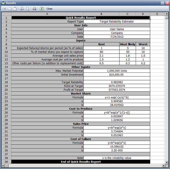
Enter the given information in the Target Reliability tool in Weibull++ and click the Plot icon on the control panel. Next, click the Analysis Details button on the control panel to generate a report of the analysis. The following report shows the cost models.
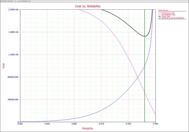
The following figure shows the Cost vs. Reliability plot of the cost models. The green vertical line on the plot represents the estimated reliability value that will minimize costs. In this example, this reliability value is estimated to be 96.7% at the end of the warranty period.
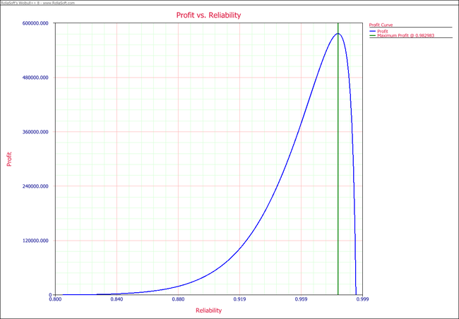
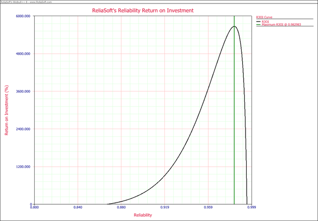
The following figures show the Profit vs. Reliability plot and the R3OI vs. Reliability plot. In the R3OI plot, the initial investment is set to $10,000.

