|
|
| (111 intermediate revisions by 9 users not shown) |
| Line 1: |
Line 1: |
| {{template:RGA BOOK|13|Fielded Systems}} | | {{template:RGA BOOK|6.1|Repairable Systems Analysis}} |
| | Data from systems in the field can be analyzed in the RGA software. This type of data is called ''fielded systems data'' and is analogous to warranty data. Fielded systems can be categorized into two basic types: one-time or non-repairable systems, and reusable or repairable systems. In the latter case, under continuous operation, the system is repaired, but not replaced after each failure. For example, if a water pump in a vehicle fails, the water pump is replaced and the vehicle is repaired. |
|
| |
|
| =Fielded Systems=
| | This chapter presents repairable systems analysis, where the reliability of a system can be tracked and quantified based on data from multiple systems in the field. The next chapter will present [[Fleet Data Analysis|fleet analysis]], where data from multiple systems in the field can be collected and analyzed so that reliability metrics for the fleet as a whole can be quantified. |
| The previous chapters presented analysis methods for data obtained during developmental testing. However, data from systems in the field can also be analyzed in RGA. This type of data is called fielded systems data and is analogous to warranty data. Fielded systems can be categorized into two basic types: one-time or nonrepairable systems and reusable or repairable systems. In the latter case, under continuous operation, the system is repaired, but not replaced after each failure. For example, if a water pump in a vehicle fails, the water pump is replaced and the vehicle is repaired.
| |
| Two types of analysis are presented in this chapter. The first is repairable systems analysis where the reliability of a system can be tracked and quantified based on data from multiple systems in the field. The second is fleet analysis where data from multiple systems in the field can be collected and analyzed so that reliability metrics for the fleet as a whole can be quantified.
| |
| ==Repairable Systems Analysis==
| |
| ===Background===
| |
| Most complex systems, such as automobiles, communication systems, aircraft, printers, medical diagnostics systems, helicopters, etc., are repaired and not replaced when they fail. When these systems are fielded or subjected to a customer use environment, it is often of considerable interest to determine the reliability and other performance characteristics under these conditions. Areas of interest may include assessing the expected number of failures during the warranty period, maintaining a minimum mission reliability, evaluating the rate of wearout, determining when to replace or overhaul a system and minimizing life cycle costs. In general, a lifetime distribution, such as the Weibull distribution, cannot be used to address these issues. In order to address the reliability characteristics of complex repairable systems, a process is often used instead of a distribution. The most popular process model is the Power Law model. This model is popular for several reasons. One is that it has a very practical foundation in terms of minimal repair. This is the situation when the repair of a failed system is just enough to get the system operational again. Second, if the time to first failure follows the Weibull distribution, then each succeeding failure is governed by the Power Law model in the case of minimal repair. From this point of view, the Power Law model is an extension of the Weibull distribution.
| |
| <br>
| |
|
| |
|
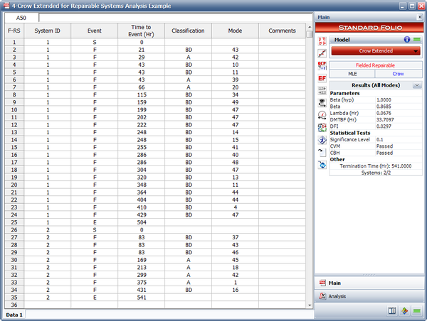
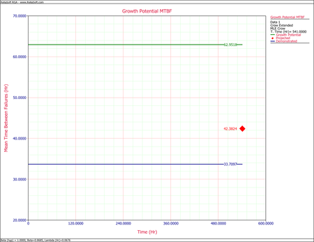
| Sometimes, the Crow Extended model , which was introduced in Chapter 9 for the developmental data, is also applied for fielded repairable systems. Applying the Crow Extended model on repairable system data allows analysts to project the system MTBF after reliability-related issues are addressed during the field operation. Projections are calculated based on the mode classifications (A, BC and BD). The calculation procedure is the same as the one for the developmental data.and is not repeated in this chapter. | | ==Background== |
| <br>
| | Most complex systems, such as automobiles, communication systems, aircraft, printers, medical diagnostics systems, helicopters, etc., are repaired and not replaced when they fail. When these systems are fielded or subjected to a customer use environment, it is often of considerable interest to determine the reliability and other performance characteristics under these conditions. Areas of interest may include assessing the expected number of failures during the warranty period, maintaining a minimum mission reliability, evaluating the rate of wearout, determining when to replace or overhaul a system and minimizing life cycle costs. In general, a lifetime distribution, such as the Weibull distribution, cannot be used to address these issues. In order to address the reliability characteristics of complex repairable systems, a process is often used instead of a distribution. The most popular process model is the Power Law model. This model is popular for several reasons. One is that it has a very practical foundation in terms of minimal repair, which is a situation where the repair of a failed system is just enough to get the system operational again. Second, if the time to first failure follows the Weibull distribution, then each succeeding failure is governed by the Power Law model as in the case of minimal repair. From this point of view, the Power Law model is an extension of the Weibull distribution. |
| | |
| | Sometimes, the [[Crow Extended]] model, which was introduced in a previous chapter for analyzing developmental data, is also applied for fielded repairable systems. Applying the Crow Extended model on repairable system data allows analysts to project the system MTBF after reliability-related issues are addressed during the field operation. Projections are calculated based on the mode classifications (A, BC and BD). The calculation procedure is the same as the one for the developmental data, and is not repeated in this chapter. |
|
| |
|
| ===Distribution Example=== | | ===Distribution Example=== |
| <br>
| | Visualize a socket into which a component is inserted at time 0. When the component fails, it is replaced immediately with a new one of the same kind. After each replacement, the socket is put back into an ''as good as new'' condition. Each component has a time-to-failure that is determined by the underlying distribution. It is important to note that a distribution relates to a single failure. The sequence of failures for the socket constitutes a random process called a ''renewal process''. In the illustration below, the component life is <math>{{X}_{j}}\,\!</math>, and <math>{{t}_{j}}\,\!</math> is the system time to the <math>{{j}^{th}}\,\!</math> failure. |
| Visualize a socket into which a component is inserted at time <math>0</math> . When the component fails, it is replaced immediately with a new one of the same kind. After each failure, the socket is put back into an ''as good as new'' condition. Each component has a time-to-failure that is determined by the underlying distribution. It is important to note that a distribution relates to a single failure. The sequence of failures for the socket constitutes a random process called a renewal process. In the illustration below, the component life is <math>{{X}_{j}}</math> and <math>{{t}_{j}}</math> is the system time to the <math>{{j}^{th}}</math> failure. | | |
|
| | [[File:Rga12.png|center|450px|Instantaneous Failure Intensity vs. Time plot.]] |
| Each component life <math>{{X}_{j}}</math> in the socket is governed by the same distribution <math>F(x)</math> .
| |
| <br>
| |
| A distribution, such as the Weibull, governs a single lifetime. There is only one event associated with a distribution. The distribution <math>F(x)</math> is the probability that the life of the component in the socket is less than <math>x</math> . In the illustration above, <math>{{X}_{1}}</math> is the life of the first component in the socket. <math>F(x)</math> is the probability that the first component in the socket fails in time <math>x</math> . When the first component fails, it is replaced in the socket with a new component of the same type. The probability that the life of the second component is less than <math>x</math> is given by the same distribution function, <math>F(x)</math> . For the Weibull distribution:
| |
|
| |
|
| | Each component life <math>{{X}_{j}}\,\!</math> in the socket is governed by the same distribution <math>F(x)\,\!</math>. |
|
| |
|
| ::<math>F(x)=1-{{e}^{-\lambda {{x}^{\beta }}}}</math>
| | A distribution, such as Weibull, governs a single lifetime. There is only one event associated with a distribution. The distribution <math>F(x)\,\!</math> is the probability that the life of the component in the socket is less than <math>x\,\!</math>. In the illustration above, <math>{{X}_{1}}\,\!</math> is the life of the first component in the socket. <math>F(x)\,\!</math> is the probability that the first component in the socket fails in time <math>x\,\!</math>. When the first component fails, it is replaced in the socket with a new component of the same type. The probability that the life of the second component is less than <math>x\,\!</math> is given by the same distribution function, <math>F(x)\,\!</math>. For the Weibull distribution: |
|
| |
|
| | :<math>F(x)=1-{{e}^{-\lambda {{x}^{\beta }}}}\,\!</math> |
|
| |
|
| A distribution is also characterized by its density function, such that: | | A distribution is also characterized by its density function, such that: |
|
| |
|
| | | :<math>f(x)=\frac{d}{dx}F(x)\,\!</math> |
| ::<math>f(x)=\frac{d}{dx}F(x)</math>
| |
| | |
|
| |
|
| The density function for the Weibull distribution is: | | The density function for the Weibull distribution is: |
|
| |
|
| | | :<math>f(x)=\lambda \beta {{x}^{\beta -1}}\cdot {{e}^{-\lambda \beta x}}\,\!</math> |
| ::<math>f(x)=\lambda \beta {{x}^{\beta -1}}\cdot {{e}^{-\lambda \beta x}}</math>
| |
| | |
|
| |
|
| In addition, an important reliability property of a distribution function is the failure rate, which is given by: | | In addition, an important reliability property of a distribution function is the failure rate, which is given by: |
|
| |
|
| | :<math>r(x)=\frac{f(x)}{1-F(x)}\,\!</math> |
|
| |
|
| ::<math>r(x)=\frac{f(x)}{1-F(x)}</math>
| | The interpretation of the failure rate is that for a small interval of time <math>\Delta x\,\!</math>, <math>r(x)\Delta x\,\!</math> is approximately the probability that a component in the socket will fail between time <math>x\,\!</math> and time <math>x+\Delta x\,\!</math>, given that the component has not failed by time <math>x\,\!</math>. For the Weibull distribution, the failure rate is given by: |
|
| |
|
| | :<math>\begin{align} |
| | r(x)=\lambda \beta {{x}^{\beta -1}} |
| | \end{align}\,\!</math> |
|
| |
|
| The interpretation of the failure rate is that for a small interval of time <math>\Delta x</math> , <math>r(x)\Delta x</math> is approximately the probability that a component in the socket will fail between time <math>x</math> and time <math>x+\Delta x</math> , given that the component has not failed by time <math>x</math> . For the Weibull distribution, the failure rate is given by:
| | It is important to note the condition that the component has not failed by time <math>x\,\!</math>. Again, a distribution deals with one lifetime of a component and does not allow for more than one failure. The socket has many failures and each failure time is individually governed by the same distribution. In other words, the failure times are independent of each other. If the failure rate is increasing, then this is indicative of component wearout. If the failure rate is decreasing, then this is indicative of infant mortality. If the failure rate is constant, then the component failures follow an exponential distribution. For the Weibull distribution, the failure rate is increasing for <math>\beta >1\,\!</math>, decreasing for <math>\beta<1\,\!</math> and constant for <math>\beta =1\,\!</math>. Each time a component in the socket is replaced, the failure rate of the new component goes back to the value at time 0. This means that the socket is as good as new after each failure and each subsequent replacement by a new component. This process is continued for the operation of the socket. |
|
| |
|
|
| |
| ::<math>r(x)=\lambda \beta {{x}^{\beta -1}}</math>
| |
|
| |
|
| |
| It is important to note the condition that the component has not failed by time <math>x</math> . Again, a distribution deals with one lifetime of a component and does not allow for more than one failure. The socket has many failures and each failure time is individually governed by the same distribution. In other words, the failure times are independent of each other. If the failure rate is increasing, then this is indicative of component wearout. If the failure rate is decreasing, then this is indicative of infant mortality. If the failure rate is constant, then the component failures follow an exponential distribution. For the Weibull distribution, the failure rate is increasing for <math>\beta >1</math> , decreasing for <math>\beta </math> <math><1</math> and constant for <math>\beta =1</math> . Each time a component in the socket is replaced, the failure rate of the new component converts back to the value at time <math>0</math> . This means that the socket is as good as new after each failure and the subsequent replacement by a new component. This process is continued for the operation of the socket.
| |
| <br>
| |
| ===Process Example=== | | ===Process Example=== |
| <br>
| | Now suppose that a system consists of many components with each component in a socket. A failure in any socket constitutes a failure of the system. Each component in a socket is a renewal process governed by its respective distribution function. When the system fails due to a failure in a socket, the component is replaced and the socket is again as good as new. The system has been repaired. Because there are many other components still operating with various ages, the system is not typically put back into a like new condition after the replacement of a single component. For example, a car is not as good as new after the replacement of a failed water pump. Therefore, distribution theory does not apply to the failures of a complex system, such as a car. In general, the intervals between failures for a complex repairable system do not follow the same distribution. Distributions apply to the components that are replaced in the sockets, but not at the system level. At the system level, a distribution applies to the very first failure. There is one failure associated with a distribution. For example, the very first system failure may follow a Weibull distribution. |
| Now suppose that a system consists of many components with each component in a socket. A failure in any socket constitutes a failure of the system. Each component in a socket is a renewal process governed by its respective distribution function. When the system fails due to a failure in a socket, the component is replaced and the socket is again as good as new. The system has been repaired. Because there are many other components still operating with various ages, the system is not typically put back into a like new condition after the replacement of a single component. For example, a car is not as good as new after the replacement of a failed water pump. Therefore, distribution theory does not apply to the failures of a complex system, such as a car. In general, the intervals between failures for a complex repairable system do not follow the same distribution. Distributions apply to the components that are replaced in the sockets but not at the system level. At the system level, a distribution applies to the very first failure. There is one failure associated with a distribution. For example, the very first system failure may follow a Weibull distribution. | |
| <br>
| |
| | |
| For many systems in a real world environment, a repair is only enough to get the system operational again. If the water pump fails on the car, the repair consists only of installing a new water pump. If a seal leaks, the seal is replaced but no additional maintenance is done, etc. This is the concept of minimal repair. For a system with many failure modes, the repair of a single failure mode does not greatly improve the system reliability from what it was just before the failure. Under minimal repair for a complex system with many failure modes, the system reliability after a repair is the same as it was just before the failure. In this case, the sequence of failure at the system level follows a non-homogeneous Poisson process (NHPP).
| |
| The system age when the system is first put into service is time <math>0</math> . Under the NHPP, the first failure is governed by a distribution <math>F(x)</math> with failure rate <math>r(x)</math> . Each succeeding failure is governed by the intensity function <math>u(t)</math> of the process. Let <math>t</math> be the age of the system and <math>\Delta t</math> is very small. The probability that a system of age <math>t</math> fails between <math>t</math> and <math>t+\Delta t</math> is given by the intensity function <math>u(t)\Delta t</math> . Notice that this probability is not conditioned on not having any system failures up to time <math>t</math> , as is the case for a failure rate. The failure intensity <math>u(t)</math> for the NHPP has the same functional form as the failure rate governing the first system failure. Therefore, <math>u(t)=r(t)</math> , where <math>r(t)</math> is the failure rate for the distribution function of the first system failure. If the first system failure follows the Weibull distribution, the failure rate is:
| |
|
| |
|
| | For many systems in a real world environment, a repair may only be enough to get the system operational again. If the water pump fails on the car, the repair consists only of installing a new water pump. Similarly, if a seal leaks, the seal is replaced but no additional maintenance is done. This is the concept of ''minimal repair''. For a system with many failure modes, the repair of a single failure mode does not greatly improve the system reliability from what it was just before the failure. Under minimal repair for a complex system with many failure modes, the system reliability after a repair is the same as it was just before the failure. In this case, the sequence of failures at the system level follows a non-homogeneous Poisson process (NHPP). |
|
| |
|
| ::<math>r(x)=\lambda \beta {{x}^{\beta -1}}</math>
| | The system age when the system is first put into service is time 0. Under the NHPP, the first failure is governed by a distribution <math>F(x)\,\!</math> with failure rate <math>r(x)\,\!</math>. Each succeeding failure is governed by the intensity function <math>u(t)\,\!</math> of the process. Let <math>t\,\!</math> be the age of the system and <math>\Delta t\,\!</math> is very small. The probability that a system of age <math>t\,\!</math> fails between <math>t\,\!</math> and <math>t+\Delta t\,\!</math> is given by the intensity function <math>u(t)\Delta t\,\!</math>. Notice that this probability is not conditioned on not having any system failures up to time <math>t\,\!</math>, as is the case for a failure rate. The failure intensity <math>u(t)\,\!</math> for the NHPP has the same functional form as the failure rate governing the first system failure. Therefore, <math>u(t)=r(t)\,\!</math>, where <math>r(t)\,\!</math> is the failure rate for the distribution function of the first system failure. If the first system failure follows the Weibull distribution, the failure rate is: |
|
| |
|
| | :<math>\begin{align} |
| | r(x)=\lambda \beta {{x}^{\beta -1}} |
| | \end{align}\,\!</math> |
|
| |
|
| Under minimal repair, the system intensity function is: | | Under minimal repair, the system intensity function is: |
|
| |
|
| | :<math>\begin{align} |
| | u(t)=\lambda \beta {{t}^{\beta -1}} |
| | \end{align}\,\!</math> |
|
| |
|
| ::<math>u(t)=\lambda \beta {{t}^{\beta -1}}</math>
| | This is the Power Law model. It can be viewed as an extension of the Weibull distribution. The Weibull distribution governs the first system failure, and the Power Law model governs each succeeding system failure. If the system has a constant failure intensity <math>u(t) = \lambda \,\!</math>, then the intervals between system failures follow an exponential distribution with failure rate <math>\lambda \,\!</math>. If the system operates for time <math>T\,\!</math>, then the random number of failures <math>N(T)\,\!</math> over 0 to <math>T\,\!</math> is given by the Power Law mean value function. |
|
| |
|
| | :<math>\begin{align} |
| | E[N(T)]=\lambda {{T}^{\beta }} |
| | \end{align}\,\!</math> |
|
| |
|
| This is the Power Law model. It can be viewed as an extension of the Weibull distribution. The Weibull distribution governs the first system failure and the Power Law model governs each succeeding system failure. If the system has a constant failure intensity <math>u(t)</math> = <math>\lambda </math> , then the intervals between system failures follow an exponential distribution with failure rate <math>\lambda </math> . If the system operates for time <math>T</math> , then the random number of failures <math>N(T)</math> over <math>0</math> to <math>T</math> is given by the Power Law mean value function.
| | Therefore, the probability <math>N(T)=n\,\!</math> is given by the Poisson probability. |
|
| |
|
| | :<math>\frac{{{\left( \lambda T \right)}^{n}}{{e}^{-\lambda T}}}{n!};\text{ }n=0,1,2\ldots \,\!</math> |
|
| |
|
| ::<math>E[N(T)]=\lambda {{T}^{\beta }}</math>
| | This is referred to as a ''homogeneous Poisson process'' because there is no change in the intensity function. This is a special case of the Power Law model for <math>\beta =1\,\!</math>. The Power Law model is a generalization of the homogeneous Poisson process and allows for change in the intensity function as the repairable system ages. For the Power Law model, the failure intensity is increasing for <math>\beta >1\,\!</math> (wearout), decreasing for <math>\beta <1\,\!</math> (infant mortality) and constant for <math>\beta =1\,\!</math> (useful life). |
|
| |
|
| | ==Power Law Model== |
| | The Power Law model is often used to analyze the reliability of complex repairable systems in the field. The system of interest may be the total system, such as a helicopter, or it may be subsystems, such as the helicopter transmission or rotator blades. When these systems are new and first put into operation, the start time is 0. As these systems are operated, they accumulate age (e.g., miles on automobiles, number of pages on copiers, flights of helicopters). When these systems fail, they are repaired and put back into service. |
|
| |
|
| Therefore, the probability <math>N(T)=n</math> is given by the Poisson probability.
| | Some system types may be overhauled and some may not, depending on the maintenance policy. For example, an automobile may not be overhauled but helicopter transmissions may be overhauled after a period of time. In practice, an overhaul may not convert the system reliability back to where it was when the system was new. However, an overhaul will generally make the system more reliable. Appropriate data for the Power Law model is over cycles. If a system is not overhauled, then there is only one cycle and the zero time is when the system is first put into operation. If a system is overhauled, then the same serial number system may generate many cycles. Each cycle will start a new zero time, the beginning of the cycle. The age of the system is from the beginning of the cycle. For systems that are not overhauled, there is only one cycle and the reliability characteristics of a system as the system ages during its life is of interest. For systems that are overhauled, you are interested in the reliability characteristics of the system as it ages during its cycle. |
|
| |
|
| | For the Power Law model, a data set for a system will consist of a starting time <math>S\,\!</math>, an ending time <math>T\,\!</math> and the accumulated ages of the system during the cycle when it had failures. Assume that the data exists from the beginning of a cycle (i.e., the starting time is 0), although non-zero starting times are possible with the Power Law model. For example, suppose data has been collected for a system with 2,000 hours of operation during a cycle. The starting time is <math>S=0\,\!</math> and the ending time is <math>T=2000\,\!</math>. Over this period, failures occurred at system ages of 50.6, 840.7, 1060.5, 1186.5, 1613.6 and 1843.4 hours. These are the accumulated operating times within the cycle, and there were no failures between 1843.4 and 2000 hours. It may be of interest to determine how the systems perform as part of a fleet. For a fleet, it must be verified that the systems have the same configuration, same maintenance policy and same operational environment. In this case, a random sample must be gathered from the fleet. Each item in the sample will have a cycle starting time <math>S=0\,\!</math>, an ending time <math>T\,\!</math> for the data period and the accumulated operating times during this period when the system failed. |
|
| |
|
| ::<math>\frac{{{\left( \lambda T \right)}^{n}}{{e}^{-\lambda T}}}{n!};\text{ }n=0,1,2\ldots </math>
| | There are many ways to generate a random sample of <math>K\,\!</math> systems. One way is to generate <math>K\,\!</math> random serial numbers from the fleet. Then go to the records corresponding to the randomly selected systems. If the systems are not overhauled, then record when each system was first put into service. For example, the system may have been put into service when the odometer mileage equaled zero. Each system may have a different amount of total usage, so the ending times, <math>T\,\!</math>, may be different. If the systems are overhauled, then the records for the last completed cycle will be needed. The starting and ending times and the accumulated times to failure for the <math>K\,\!</math> systems constitute the random sample from the fleet. There is a useful and efficient method for generating a random sample for systems that are overhauled. If the overhauled systems have been in service for a considerable period of time, then each serial number system in the fleet would go through many overhaul cycles. In this case, the systems coming in for overhaul actually represent a random sample from the fleet. As <math>K\,\!</math> systems come in for overhaul, the data for the current completed cycles would be a random sample of size <math>K\,\!</math>. |
|
| |
|
| | In addition, the warranty period may be of particular interest. In this case, randomly choose <math>K\,\!</math> serial numbers for systems that have been in customer use for a period longer than the warranty period. Then check the warranty records. For each of the <math>K\,\!</math> systems that had warranty work, the ages corresponding to this service are the failure times. If a system did not have warranty work, then the number of failures recorded for that system is zero. The starting times are all equal to zero and the ending time for each of the <math>K\,\!</math> systems is equal to the warranty operating usage time (e.g., hours, copies, miles). |
|
| |
|
| This is referred to as a homogeneous Poisson process because there is no change in the intensity function. This is a special case of the Power Law model for <math>\beta =1</math> . The Power Law model is a generalization of the homogeneous Poisson process and allows for change in the intensity function as the repairable system ages. For the Power Law model, the failure intensity is increasing for <math>\beta >1</math> (wearout), decreasing for <math>\beta <1</math> (infant morality) and constant for <math>\beta =1</math> (useful life).
| | In addition to the intensity function <math>u(t)\,\!</math> and the mean value function, which were given in the [[Repairable Systems Analysis#Process_Example|section above]], other relationships based on the Power Law are often of practical interest. For example, the probability that the system will survive to age <math>t+d\,\!</math> without failure is given by: |
| <br>
| |
|
| |
|
| ===Using the Power Law Model to Analyze Complex Repairable Systems===
| | :<math>R(t)={{e}^{-\left[ \lambda {{\left( t+d \right)}^{\beta }}-\lambda {{t}^{\beta }} \right]}}\,\!</math> |
| <br> | |
| The Power Law model is often used to analyze the reliability for complex repairable systems in the field. A system of interest may be the total system, such as a helicopter, or it may be subsystems, such as the helicopter transmission or rotator blades. When these systems are new and first put into operation, the start time is <math>0</math> . As these systems are operated, they accumulate age, e.g. miles on automobiles, number of pages on copiers, hours on helicopters. When these systems fail, they are repaired and put back into service.
| |
| <br>
| |
|
| |
|
| Some system types may be overhauled and some may not, depending on the maintenance policy. For example, an automobile may not be overhauled but helicopter transmissions may be overhauled after a period of time. In practice, an overhaul may not convert the system reliability back to where it was when the system was new.
| | This is the mission reliability for a system of age <math>t\,\!</math> and mission length <math>d\,\!</math>. |
| However, an overhaul will generally make the system more reliable. Appropriate data for the Power Law model is over cycles. If a system is not overhauled, then there is only one cycle and the zero time is when the system is first put into operation. If a system is overhauled, then the same serial number system may generate many cycles. Each cycle will start a new zero time, the beginning of the cycle. The age of the system is from the beginning of the cycle. For systems that are not overhauled, there is only one cycle and the reliability characteristics of a system as the system ages during its life is of interest. For systems that are overhauled, you are interested in the reliability characteristics of the system as it ages during its cycle.
| |
| <br> | |
|
| |
|
| For the Power Law model, a data set for a system will consist of a starting time <math>S</math> , an ending time <math>T</math> and the accumulated ages of the system during the cycle when it had failures. Assume the data exists from the beginning of a cycle (i.e. the starting time is 0), although non-zero starting times are possible with the Power Law model. For example, suppose data has been collected for a system with 2000 hours of operation during a cycle. The starting time is <math>S=0</math> and the ending time is <math>T=2000</math> . Over this period, failures occurred at system ages of 50.6, 840.7, 1060.5, 1186.5, 1613.6 and 1843.4 hours. These are the accumulated operating times within the cycle and there were no failures between 1843.4 and 2000 hours. It may be of interest to determine how the systems perform as part of a fleet. For a fleet, it must be verified that the systems have the same configuration, same maintenance policy and same operational environment. In this case, a random sample must be gathered from the fleet. Each item in the sample will have a cycle starting time <math>S=0</math> , an ending time <math>T</math> for the data period and the accumulated operating times during this period when the system failed.
| | ===Parameter Estimation=== |
| <br> | | Suppose that the number of systems under study is <math>K\,\!</math> and the <math>{{q}^{th}}\,\!</math> system is observed continuously from time <math>{{S}_{q}}\,\!</math> to time <math>{{T}_{q}}\,\!</math>, <math>q=1,2,\ldots ,K\,\!</math>. During the period <math>[{{S}_{q}},{{T}_{q}}]\,\!</math>, let <math>{{N}_{q}}\,\!</math> be the number of failures experienced by the <math>{{q}^{th}}\,\!</math> system and let <math>{{X}_{i,q}}\,\!</math> be the age of this system at the <math>{{i}^{th}}\,\!</math> occurrence of failure, <math>i=1,2,\ldots ,{{N}_{q}}\,\!</math>. It is also possible that the times <math>{{S}_{q}}\,\!</math> and <math>{{T}_{q}}\,\!</math> may be the observed failure times for the <math>{{q}^{th}}\,\!</math> system. If <math>{{X}_{{{N}_{q}},q}}={{T}_{q}}\,\!</math>, then the data on the <math>{{q}^{th}}\,\!</math> system is said to be failure terminated, and <math>{{T}_{q}}\,\!</math> is a random variable with <math>{{N}_{q}}\,\!</math> fixed. If <math>{{X}_{{{N}_{q}},q}}<{{T}_{q}}\,\!</math>, then the data on the <math>{{q}^{th}}\,\!</math> system is said to be time terminated with <math>{{N}_{q}}\,\!</math> a random variable. The maximum likelihood estimates of <math>\lambda \,\!</math> and <math>\beta \,\!</math> are values satisfying the equations shown next. |
|
| |
|
| There are many ways to generate a random sample of <math>K</math> systems. One way is to generate <math>K</math> random serial numbers from the fleet. Then go to the records corresponding to the randomly selected systems. If the systems are not overhauled, then record when each system was first put into service. For example, the system may have been put into service when the odometer mileage equaled zero. Each system may have a different amount of total usage, so the ending times, <math>T</math> , may be different. If the systems are overhauled, then the records for the last completed cycle will be needed. The starting and ending times and the accumulated times to failure for the <math>K</math> systems constitute the random sample from the fleet. There is a useful and efficient method for generating a random sample for systems that are overhauled. If the overhauled systems have been in service for a considerable period of time, then each serial number system in the fleet would go through many overhaul cycles. In this case, the systems coming in for overhaul actually represent a random sample from the fleet. As <math>K</math> systems come in for overhaul, the data for the current completed cycles would be a random sample of size <math>K</math> .
| | :<math>\begin{align} |
| <br>
| | \widehat{\lambda }= & \frac{\underset{q=1}{\overset{K}{\mathop{\sum }}}\,{{N}_{q}}}{\underset{q=1}{\overset{K}{\mathop{\sum }}}\,\left( T_{q}^{\widehat{\beta }}-S_{q}^{\widehat{\beta }} \right)} \\ |
| | \widehat{\beta }= & \frac{\underset{q=1}{\overset{K}{\mathop{\sum }}}\,{{N}_{q}}}{\widehat{\lambda }\underset{q=1}{\overset{K}{\mathop{\sum }}}\,\left[ T_{q}^{\widehat{\beta }}\ln ({{T}_{q}})-S_{q}^{\widehat{\beta }}\ln ({{S}_{q}}) \right]-\underset{q=1}{\overset{K}{\mathop{\sum }}}\,\underset{i=1}{\overset{{{N}_{q}}}{\mathop{\sum }}}\,\ln ({{X}_{i,q}})} |
| | \end{align}\,\!</math> |
|
| |
|
| In addition, the warranty period may be of particular interest. In this case, randomly choose <math>K</math> serial numbers for systems that have been in customer use for a period longer than the warranty period. Then check the warranty records. For each of the <math>K</math> systems that had warranty work, the ages corresponding to this service are the failure times. If a system did not have warranty work, then the number of failures recorded for that system is zero. The starting times are all equal to zero and the ending time for each of the <math>K</math> systems is equal to the warranty operating usage time, e.g. hours, copies, miles.
| | where <math>0\ln 0\,\!</math> is defined to be 0. In general, these equations cannot be solved explicitly for <math>\widehat{\lambda }\,\!</math> and <math>\widehat{\beta },\,\!</math> but must be solved by iterative procedures. Once <math>\widehat{\lambda }\,\!</math> and <math>\widehat{\beta }\,\!</math> have been estimated, the maximum likelihood estimate of the intensity function is given by: |
| In addition to the intensity function <math>u(t)</math> given by Eqn. (intensity) and the mean value function given by Eqn. (expected failures), other relationships based on the Power Law are often of practical interest. For example, the probability that the system will survive to age <math>t+d</math> without failure is given by:
| |
|
| |
|
| | :<math>\widehat{u}(t)=\widehat{\lambda }\widehat{\beta }{{t}^{\widehat{\beta }-1}}\,\!</math> |
|
| |
|
| ::<math>R(t)={{e}^{-\left[ \lambda {{\left( t+d \right)}^{\beta }}-\lambda {{t}^{\beta }} \right]}}</math>
| | If <math>{{S}_{1}}={{S}_{2}}=\ldots ={{S}_{q}}=0\,\!</math> and <math>{{T}_{1}}={{T}_{2}}=\ldots ={{T}_{q}}\,\!</math> <math>\,(q=1,2,\ldots ,K)\,\!</math> then the maximum likelihood estimates <math>\widehat{\lambda }\,\!</math> and <math>\widehat{\beta }\,\!</math> are in closed form. |
|
| |
|
| | :<math>\begin{align} |
| | \widehat{\lambda }= & \frac{\underset{q=1}{\overset{K}{\mathop{\sum }}}\,{{N}_{q}}}{K{{T}^{\beta }}} \\ |
| | \widehat{\beta }= & \frac{\underset{q=1}{\overset{K}{\mathop{\sum }}}\,{{N}_{q}}}{\underset{q=1}{\overset{K}{\mathop{\sum }}}\,\underset{i=1}{\overset{{{N}_{q}}}{\mathop{\sum }}}\,\ln (\tfrac{T}{{{X}_{iq}}})} |
| | \end{align}\,\!</math> |
|
| |
|
| This is the mission reliability for a system of age <math>t</math> and mission length <math>d</math> .
| | The following example illustrates these estimation procedures. |
| <br>
| |
|
| |
|
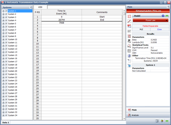
| ==Parameter Estimation== | | ===Power Law Model Example=== <!-- THIS SECTION HEADER IS LINKED FROM ANOTHER SECTION IN THIS DOCUMENT. IF YOU RENAME THE SECTION, YOU MUST UPDATE THE LINK(S). --> |
| <br>
| | {{:Power Law Model Parameter Estimation Example}} |
| Suppose that the number of systems under study is <math>K</math> and the <math>{{q}^{th}}</math> system is observed continuously from time <math>{{S}_{q}}</math> to time <math>{{T}_{q}}</math> , <math>q=1,2,\ldots ,K</math> . During the period <math>[{{S}_{q}},{{T}_{q}}]</math> , let <math>{{N}_{q}}</math> be the number of failures experienced by the <math>{{q}^{th}}</math> system and let <math>{{X}_{i,q}}</math> be the age of this system at the <math>{{i}^{th}}</math> occurrence of failure, <math>i=1,2,\ldots ,{{N}_{q}}</math> . It is also possible that the times <math>{{S}_{q}}</math> and <math>{{T}_{q}}</math> may be observed failure times for the <math>{{q}^{th}}</math> system. If <math>{{X}_{{{N}_{q}},q}}={{T}_{q}}</math> then the data on the <math>{{q}^{th}}</math> system is said to be failure terminated and <math>{{T}_{q}}</math> is a random variable with <math>{{N}_{q}}</math> fixed. If <math>{{X}_{{{N}_{q}},q}}<{{T}_{q}}</math> then the data on the <math>{{q}^{th}}</math> system is said to be time terminated with <math>{{N}_{q}}</math> a random variable. The maximum likelihood estimates of <math>\lambda </math> and <math>\beta </math> are values satisfying the Eqns. (lambdaPowerLaw) and (BetaPowerLaw).
| |
|
| |
|
| | ==Goodness-of-Fit Tests for Repairable System Analysis==<!-- THIS SECTION HEADER IS LINKED TO: Hypothesis Tests. IF YOU RENAME THE SECTION, YOU MUST UPDATE THE LINK. --> |
| | It is generally desirable to test the compatibility of a model and data by a statistical goodness-of-fit test. A parametric Cramér-von Mises goodness-of-fit test is used for the multiple system and repairable system Power Law model, as proposed by Crow in [[RGA_References|[17]]]. This goodness-of-fit test is appropriate whenever the start time for each system is 0 and the failure data is complete over the continuous interval <math>[0,{{T}_{q}}]\,\!</math> with no gaps in the data. The Chi-Squared test is a goodness-of-fit test that can be applied under more general circumstances. In addition, the Common Beta Hypothesis test also can be used to compare the intensity functions of the individual systems by comparing the <math>{{\beta }_{q}}\,\!</math> values of each system. Lastly, the Laplace Trend test checks for trends within the data. Due to their general application, the Common Beta Hypothesis test and the Laplace Trend test are both presented in [[Hypothesis_Tests|Appendix B]]. The Cramér-von Mises and Chi-Squared goodness-of-fit tests are illustrated next. |
|
| |
|
| ::<math>\begin{align}
| | ===Cramér-von Mises Test=== |
| & \widehat{\lambda }= & \frac{\underset{q=1}{\overset{K}{\mathop{\sum }}}\,{{N}_{q}}}{\underset{q=1}{\overset{K}{\mathop{\sum }}}\,\left( T_{q}^{\widehat{\beta }}-S_{q}^{\widehat{\beta }} \right)} \\
| | To illustrate the application of the Cramér-von Mises statistic for multiple systems data, suppose that <math>K\,\!</math> like systems are under study and you wish to test the hypothesis <math>{{H}_{1}}\,\!</math> that their failure times follow a non-homogeneous Poisson process. Suppose information is available for the <math>{{q}^{th}}\,\!</math> system over the interval <math>[0,{{T}_{q}}]\,\!</math>, with successive failure times , <math>(q=1,2,\ldots ,\,K)\,\!</math>. The Cramér-von Mises test can be performed with the following steps: |
| & \widehat{\beta }= & \frac{\underset{q=1}{\overset{K}{\mathop{\sum }}}\,{{N}_{q}}}{\widehat{\lambda }\underset{q=1}{\overset{K}{\mathop{\sum }}}\,\left[ T_{q}^{\widehat{\beta }}\ln ({{T}_{q}})-S_{q}^{\widehat{\beta }}\ln ({{S}_{q}}) \right]-\underset{q=1}{\overset{K}{\mathop{\sum }}}\,\underset{i=1}{\overset{{{N}_{q}}}{\mathop{\sum }}}\,\ln ({{X}_{i,q}})}
| |
| \end{align}</math> | |
|
| |
|
| | '''Step 1:''' If <math>{{x}_{{{N}_{q}}q}}={{T}_{q}}\,\!</math> (failure terminated), let <math>{{M}_{q}}={{N}_{q}}-1\,\!</math>, and if <math>{{x}_{{{N}_{q}}q}}<T\,\!</math> (time terminated), let <math>{{M}_{q}}={{N}_{q}}\,\!</math>. Then: |
|
| |
|
| where <math>0\ln 0</math> is defined to be 0. In general, these equations cannot be solved explicitly for <math>\widehat{\lambda }</math> and <math>\widehat{\beta },</math> but must be solved by iterative procedures. Once <math>\widehat{\lambda }</math> and <math>\widehat{\beta }</math> have been estimated, the maximum likelihood estimate of the intensity function is given by:
| | :<math>M=\underset{q=1}{\overset{K}{\mathop \sum }}\,{{M}_{q}}\,\!</math> |
|
| |
|
| ::<math>\widehat{u}(t)=\widehat{\lambda }\widehat{\beta }{{t}^{\widehat{\beta }-1}}</math> | | '''Step 2:''' For each system, divide each successive failure time by the corresponding end time <math>{{T}_{q}}\,\!</math>, <math>\,i=1,2,...,{{M}_{q}}.\,\!</math> Calculate the <math>M\,\!</math> values: |
|
| |
|
| If <math>{{S}_{1}}={{S}_{2}}=\ldots ={{S}_{q}}=0</math> and <math>{{T}_{1}}={{T}_{2}}=\ldots ={{T}_{q}}</math> <math>\,(q=1,2,\ldots ,K)</math> then the maximum likelihood estimates <math>\widehat{\lambda }</math> and <math>\widehat{\beta }</math> are in closed form.
| | :<math>{{Y}_{iq}}=\frac{{{X}_{iq}}}{{{T}_{q}}},i=1,2,\ldots ,{{M}_{q}},\text{ }q=1,2,\ldots ,K\,\!</math> |
|
| |
|
| ::<math>\begin{align} | | '''Step 3:''' Next calculate <math>\bar{\beta }\,\!</math>, the unbiased estimate of <math>\beta \,\!</math>, from: |
| & \widehat{\lambda }= & \frac{\underset{q=1}{\overset{K}{\mathop{\sum }}}\,{{N}_{q}}}{K{{T}^{\beta }}} \\
| |
| & \widehat{\beta }= & \frac{\underset{q=1}{\overset{K}{\mathop{\sum }}}\,{{N}_{q}}}{\underset{q=1}{\overset{K}{\mathop{\sum }}}\,\underset{i=1}{\overset{{{N}_{q}}}{\mathop{\sum }}}\,\ln (\tfrac{T}{{{X}_{iq}}})}
| |
| \end{align}</math>
| |
|
| |
|
| | :<math>\bar{\beta }=\frac{M-1}{\underset{q=1}{\overset{K}{\mathop{\sum }}}\,\underset{i=1}{\overset{Mq}{\mathop{\sum }}}\,\ln \left( \tfrac{{{T}_{q}}}{{{X}_{i}}{{}_{q}}} \right)}\,\!</math> |
|
| |
|
| The following examples illustrate these estimation procedures.
| | '''Step 4:''' Treat the <math>{{Y}_{iq}}\,\!</math> values as one group, and order them from smallest to largest. Name these ordered values <math>{{z}_{1}},\,{{z}_{2}},\ldots ,{{z}_{M}}\,\!</math>, such that <math>{{z}_{1}}<\ \ {{z}_{2}}<\ldots <{{z}_{M}}\,\!</math>. |
| <br>
| |
| <br>
| |
| =====Example 1=====
| |
| <br>
| |
| For the data in Table 13.1, the starting time for each system is equal to <math>0</math> and the ending time for each system is 2000 hours. Calculate the maximum likelihood estimates <math>\widehat{\lambda }</math> and <math>\widehat{\beta }</math> .
| |
|
| |
|
| <br>
| | '''Step 5:''' Calculate the parametric Cramér-von Mises statistic. |
| {|system= align="center" border="1"
| |
| |-
| |
| |colspan="3" style="text-align:center"|Table 13.1 - Repairable system failure data
| |
| |-
| |
| !System 1 ( <math>{{X}_{i1}}</math> )
| |
| !System 2 ( <math>{{X}_{i2}}</math> )
| |
| !System 3 ( <math>{{X}_{i3}}</math> )
| |
| |-
| |
| |1.2|| 1.4|| 0.3
| |
| |-
| |
| |55.6|| 35.0|| 32.6
| |
| |-
| |
| |72.7|| 46.8|| 33.4
| |
| |-
| |
| |111.9|| 65.9|| 241.7
| |
| |-
| |
| |121.9|| 181.1|| 396.2
| |
| |-
| |
| |303.6|| 712.6|| 444.4
| |
| |-
| |
| |326.9|| 1005.7|| 480.8
| |
| |-
| |
| |1568.4|| 1029.9 ||588.9
| |
| |-
| |
| |1913.5|| 1675.7|| 1043.9
| |
| |-
| |
| | ||1787.5|| 1136.1
| |
| |-
| |
| | ||1867.0|| 1288.1
| |
| |-
| |
| | || ||1408.1
| |
| |-
| |
| | || ||1439.4
| |
| |-
| |
| | || ||1604.8
| |
| |-
| |
| |<math>{{N}_{1}}=9</math> || <math>{{N}_{2}}=11</math> ||<math>{{N}_{3}}=14</math>
| |
| |}
| |
|
| |
|
| <br> | | :<math>C_{M}^{2}=\frac{1}{12M}+\underset{j=1}{\overset{M}{\mathop \sum }}\,{{(Z_{j}^{\overline{\beta }}-\frac{2j-1}{2M})}^{2}}\,\!</math> |
| '''Solution'''
| |
| <br>
| |
| Since the starting time for each system is equal to zero and each system has an equivalent ending time, the general Eqns. (lambdaPowerLaw) and (BetaPowerLaw) reduce to the closed form Eqns. (sample1) and (sample2). The maximum likelihood estimates of <math>\hat{\beta }</math> and <math>\hat{\lambda }</math> are then calculated as follows:
| |
|
| |
|
| ::<math>\begin{align}
| | Critical values for the Cramér-von Mises test are presented in the [[Crow-AMSAA (NHPP)#Critical_Values|Crow-AMSAA (NHPP)]] page. |
| & \widehat{\beta }= & \frac{\underset{q=1}{\overset{K}{\mathop{\sum }}}\,{{N}_{q}}}{\underset{q=1}{\overset{K}{\mathop{\sum }}}\,\underset{i=1}{\overset{{{N}_{q}}}{\mathop{\sum }}}\,\ln (\tfrac{T}{{{X}_{iq}}})} \\
| |
| & = & 0.45300
| |
| \end{align}</math>
| |
|
| |
|
| | '''Step 6:''' If the calculated <math>C_{M}^{2}\,\!</math> is less than the critical value, then accept the hypothesis that the failure times for the <math>K\,\!</math> systems follow the non-homogeneous Poisson process with intensity function <math>u(t)=\lambda \beta {{t}^{\beta -1}}\,\!</math>. |
|
| |
|
| ::<math>\begin{align}
| | ===Chi-Squared Test=== |
| & \widehat{\lambda }= & \frac{\underset{q=1}{\overset{K}{\mathop{\sum }}}\,{{N}_{q}}}{K{{T}^{\beta }}} \\
| | The parametric Cramér-von Mises test described above requires that the starting time, <math>{{S}_{q}}\,\!</math>, be equal to 0 for each of the <math>K\,\!</math> systems. Although not as powerful as the Cramér-von Mises test, the chi-squared test can be applied regardless of the starting times. The expected number of failures for a system over its age <math>(a,b)\,\!</math> for the chi-squared test is estimated by <math>\widehat{\lambda }{{b}^{\widehat{\beta }}}-\widehat{\lambda }{{a}^{\widehat{\beta }}}=\widehat{\theta }\,\!</math>, where <math>\widehat{\lambda }\,\!</math> and <math>\widehat{\beta }\,\!</math> are the maximum likelihood estimates. |
| & = & 0.36224
| |
| \end{align}</math> | |
|
| |
|
| | The computed <math>{{\chi }^{2}}\,\!</math> statistic is: |
|
| |
|
| [[Image:rga13.2.png|thumb|center|300px|Instantaneous Failure Intensity vs. Time plot.]]
| | :<math>{{\chi }^{2}}=\underset{j=1}{\overset{d}{\mathop \sum }}\,{{\frac{\left[ N(j)-\theta (j) \right]}{\widehat{\theta }(j)}}^{2}}\,\!</math> |
|
| |
|
| <br> | | where <math>d\,\!</math> is the total number of intervals. The random variable <math>{{\chi }^{2}}\,\!</math> is approximately chi-square distributed with <math>df=d-2\,\!</math> degrees of freedom. There must be at least three intervals and the length of the intervals do not have to be equal. It is common practice to require that the expected number of failures for each interval, <math>\theta (j)\,\!</math>, be at least five. If <math>\chi _{0}^{2}>\chi _{\alpha /2,d-2}^{2}\,\!</math> or if <math>\chi _{0}^{2}<\chi _{1-(\alpha /2),d-2}^{2}\,\!</math>, reject the null hypothesis. |
| The system failure intensity function is then estimated by: | |
|
| |
|
| ::<math>\widehat{u}(t)=\widehat{\lambda }\widehat{\beta }{{t}^{\widehat{\beta }-1}},\text{ }t>0</math>
| | ===Cramér-von Mises Example=== |
| | For the data from [[Repairable Systems Analysis#Power_Law_Model_Example|power law model example]] given above, use the Cramér-von Mises test to examine the compatibility of the model at a significance level <math>\alpha =0.10\,\!</math> |
|
| |
|
| Figure wpp intensity is a plot of <math>\widehat{u}(t)</math> over the period (0, 3000). Clearly, the estimated failure intensity function is most representative over the range of the data and any extrapolation should be viewed with the usual caution.
| | '''Solution''' |
| | |
| ===Goodness-of-Fit Tests for Repairable System Analysis===
| |
| <br>
| |
| It is generally desirable to test the compatibility of a model and data by a statistical goodness-of-fit test. A parametric Cramér-von Mises goodness-of-fit test is used for the multiple system and repairable system Power Law model, as proposed by Crow in [17]. This goodness-of-fit test is appropriate whenever the start time for each system is 0 and the failure data is complete over the continuous interval <math>[0,{{T}_{q}}]</math> with no gaps in the data. The Chi-Squared test is a goodness-of-fit test that can be applied under more general circumstances. In addition, the Common Beta Hypothesis test also can be used to compare the intensity functions of the individual systems by comparing the <math>{{\beta }_{q}}</math> values of each system. Lastly, the Laplace Trend test checks for trends within the data. Due to their general applicatoin, the Common Beta Hypothesis test and the Laplace Trend test are both presented in Appendix B. The Cramér-von Mises and Chi-Squared goodness-of-fit tests are illustrated next.
| |
| <br>
| |
| <br>
| |
| ====Cramér-von Mises Test====
| |
| <br>
| |
| To illustrate the application of the Cramér-von Mises statistic for multiple system data, suppose that <math>K</math> like systems are under study and you wish to test the hypothesis <math>{{H}_{1}}</math> that their failure times follow a non-homogeneous Poisson process. Suppose information is available for the <math>{{q}^{th}}</math> system over the interval <math>[0,{{T}_{q}}]</math> , with successive failure times , <math>(q=1,2,\ldots ,\,K)</math> . The Cramér-von Mises test can be performed with the following steps:
| |
| <br>
| |
| <br>
| |
| Step 1: If <math>{{x}_{{{N}_{q}}q}}={{T}_{q}}</math> (failure terminated) let <math>{{M}_{q}}={{N}_{q}}-1</math> , and if <math>{{x}_{{{N}_{q}}q}}<T</math> (time terminated) let <math>{{M}_{q}}={{N}_{q}}</math> . Then:
| |
| | |
| ::<math>M=\underset{q=1}{\overset{K}{\mathop \sum }}\,{{M}_{q}}</math>
| |
| | |
| Step 2: For each system divide each successive failure time by the corresponding end time <math>{{T}_{q}}</math> , <math>\,i=1,2,...,{{M}_{q}}.</math> Calculate the <math>M</math> values:
| |
| | |
| ::<math>{{Y}_{iq}}=\frac{{{X}_{iq}}}{{{T}_{q}}},i=1,2,\ldots ,{{M}_{q}},\text{ }q=1,2,\ldots ,K</math>
| |
|
| |
|
| | '''Step 1''': |
|
| |
|
| Step 3: Next calculate <math>\overline{\beta }</math> , the unbiased estimate of <math>\beta </math> , from:
| | :<math>\begin{align} |
| | {{X}_{9,1}}= & 1913.5<2000,\,\ {{M}_{1}}=9 \\ |
| | {{X}_{11,2}}= & 1867<2000,\,\ {{M}_{2}}=11 \\ |
| | {{X}_{14,3}}= & 1604.8<2000,\,\ {{M}_{3}}=14 \\ |
| | M= & \underset{q=1}{\overset{3}{\mathop \sum }}\,{{M}_{q}}=34 |
| | \end{align}\,\!</math> |
|
| |
|
| ::<math>\overline{\beta }=\frac{M-1}{\underset{q=1}{\overset{K}{\mathop{\sum }}}\,\underset{i=1}{\overset{Mq}{\mathop{\sum }}}\,\ln \left( \tfrac{{{T}_{q}}}{{{X}_{i}}{{}_{q}}} \right)}</math> | | '''Step 2''': Calculate <math>{{Y}_{iq}},\,\!</math> treat the <math>{{Y}_{iq}}\,\!</math> values as one group and order them from smallest to largest. Name these ordered values <math>{{z}_{1}},\,{{z}_{2}},\ldots ,{{z}_{M}}\,\!</math>. |
|
| |
|
| | '''Step 3''': Calculate: |
|
| |
|
| Step 4: Treat the <math>{{Y}_{iq}}</math> values as one group and order them from smallest to largest. Name these ordered values <math>{{z}_{1}},\,{{z}_{2}},\ldots ,{{z}_{M}}</math> , such that <math>{{z}_{1}}<\ \ {{z}_{2}}<\ldots <{{z}_{M}}</math> .
| | :<math>\bar{\beta }=\tfrac{M-1}{\underset{q=1}{\overset{K}{\mathop{\sum }}}\,\underset{i=1}{\overset{Mq}{\mathop{\sum }}}\,\ln \left( \tfrac{{{T}_{q}}}{{{X}_{i}}{{}_{q}}} \right)}=0.4397\,\!</math> |
| <br>
| |
| <br>
| |
| Step 5: Calculate the parametric Cramér-von Mises statistic.
| |
|
| |
|
| ::<math>C_{M}^{2}=\frac{1}{12M}+\underset{j=1}{\overset{M}{\mathop \sum }}\,{{(Z_{j}^{\overline{\beta }}-\frac{2j-1}{2M})}^{2}}</math> | | '''Step 4''': Calculate: |
|
| |
|
| | :<math>C_{M}^{2}=\tfrac{1}{12M}+\underset{j=1}{\overset{M}{\mathop{\sum }}}\,{{(Z_{j}^{\overline{\beta }}-\tfrac{2j-1}{2M})}^{2}}=0.0636\,\!</math> |
|
| |
|
| Critical values for the Cramér-von Mises test are presented in Table B.2 of Appendix B.
| | '''Step 5''': From the [[Crow-AMSAA (NHPP)#Critical_Values|table of critical values for the Cramér-von Mises test]], find the critical value (CV) for <math>M=34\,\!</math> at a significance level <math>\alpha =0.10\,\!</math>. <math>CV=0.172\,\!</math>. |
| <br>
| |
| <br>
| |
| Step 6: If the calculated <math>C_{M}^{2}</math> is less than the critical value then accept the hypothesis that the failure times for the <math>K</math> systems follow the non-homogeneous Poisson process with intensity function <math>u(t)=\lambda \beta {{t}^{\beta -1}}</math> .
| |
| <br>
| |
| <br>
| |
| =====Example 2=====
| |
| <br>
| |
| For the data from Example 1, use the Cramér-von Mises test to examine the compatibility of the model at a significance level <math>\alpha =0.10</math>
| |
| <br> | |
| <br> | |
| ''Solution''
| |
| <br>
| |
| Step 1:
| |
|
| |
|
| ::<math>\begin{align} | | '''Step 6''': Since <math>C_{M}^{2}<CV\,\!</math>, accept the hypothesis that the failure times for the <math>K=3\,\!</math> repairable systems follow the non-homogeneous Poisson process with intensity function <math>u(t)=\lambda \beta {{t}^{\beta -1}}\,\!</math>. |
| & {{X}_{9,1}}= & 1913.5<2000,\,\ {{M}_{1}}=9 \\
| |
| & {{X}_{11,2}}= & 1867<2000,\,\ {{M}_{2}}=11 \\
| |
| & {{X}_{14,3}}= & 1604.8<2000,\,\ {{M}_{3}}=14 \\
| |
| & M= & \underset{q=1}{\overset{3}{\mathop \sum }}\,{{M}_{q}}=34
| |
| \end{align}</math> | |
|
| |
|
| | ==Confidence Bounds for Repairable Systems Analysis== |
| | The RGA software provides two methods to estimate the confidence bounds for repairable systems analysis. The Fisher matrix approach is based on the Fisher information matrix and is commonly employed in the reliability field. The Crow bounds were developed by Dr. Larry Crow. See [[Confidence Bounds for Repairable Systems Analysis]] for details on how these confidence bounds are calculated. |
|
| |
|
| Step 2: Calculate <math>{{Y}_{iq}},</math> treat the <math>{{Y}_{iq}}</math> values as one group and order them from smallest to largest. Name these ordered values <math>{{z}_{1}},\,{{z}_{2}},\ldots ,{{z}_{M}}</math> .
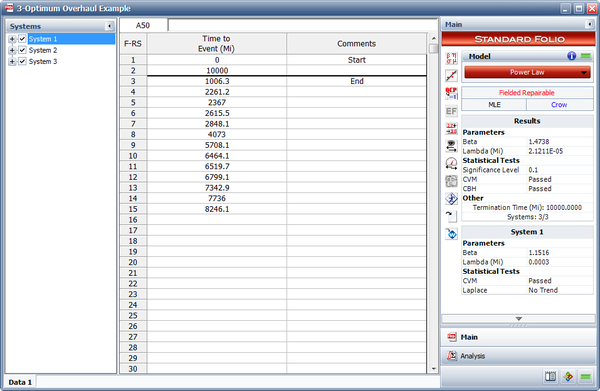
| | ===Confidence Bounds Example=== |
| <br>
| | {{:Power_Law_Model_Confidence_Bounds_Example}} |
| <br>
| |
| Step 3: Calculate <math>\overline{\beta }=\tfrac{M-1}{\underset{q=1}{\overset{K}{\mathop{\sum }}}\,\underset{i=1}{\overset{Mq}{\mathop{\sum }}}\,\ln \left( \tfrac{{{T}_{q}}}{{{X}_{i}}{{}_{q}}} \right)}=0.4397</math>
| |
| <br>
| |
| <br>
| |
| Step 4: Calculate <math>C_{M}^{2}=\tfrac{1}{12M}+\underset{j=1}{\overset{M}{\mathop{\sum }}}\,{{(Z_{j}^{\overline{\beta }}-\tfrac{2j-1}{2M})}^{2}}=0.0611</math>
| |
| <br>
| |
| <br>
| |
| Step 5: Find the critical value (CV) from Table B.2 for <math>M=34</math> at a significance level <math>\alpha =0.10</math> . <math>CV=0.172</math> .
| |
| <br>
| |
| <br>
| |
| Step 6: Since <math>C_{M}^{2}<CV</math> , accept the hypothesis that the failure times for the <math>K=3</math> repairable systems follow the non-homogeneous Poisson process with intensity function <math>u(t)=\lambda \beta {{t}^{\beta -1}}</math> .
| |
| <br>
| |
| <br>
| |
|
| |
|
| ====Chi-Squared Test==== | | ==Economical Life Model== |
| <br>
| | One consideration in reducing the cost to maintain repairable systems is to establish an overhaul policy that will minimize the total life cost of the system. However, an overhaul policy makes sense only if <math>\beta >1\,\!</math>. It does not make sense to implement an overhaul policy if <math>\beta <1\,\!</math> since wearout is not present. If you assume that there is a point at which it is cheaper to overhaul a system than to continue repairs, what is the overhaul time that will minimize the total life cycle cost while considering repair cost and the cost of overhaul? |
| The parametric Cramér-von Mises test described above requires that the starting time, <math>{{S}_{q}}</math> , be equal to 0 for each of the <math>K</math> systems. Although not as powerful as the Cramér-von Mises test, the Chi-Squared test can be applied regardless of the starting times. The expected number of failures for a system over its age <math>(a,b)</math> for the Chi-Squared test is estimated by <math>\widehat{\lambda }{{b}^{\widehat{\beta }}}-\widehat{\lambda }{{a}^{\widehat{\beta }}}=\widehat{\theta }</math> , where <math>\widehat{\lambda }</math> and <math>\widehat{\beta }</math> are the maximum likelihood estimates.
| |
| The computed <math>{{\chi }^{2}}</math> statistic is:
| |
|
| |
|
| ::<math>{{\chi }^{2}}=\underset{j=1}{\overset{d}{\mathop \sum }}\,{{\frac{\left[ N(j)-\theta (j) \right]}{\widehat{\theta }(j)}}^{2}}</math>
| | Denote <math>{{C}_{1}}\,\!</math> as the average repair cost (unscheduled), <math>{{C}_{2}}\,\!</math> as the replacement or overhaul cost and <math>{{C}_{3}}\,\!</math> as the average cost of scheduled maintenance. Scheduled maintenance is performed for every <math>S\,\!</math> miles or time interval. In addition, let <math>{{N}_{1}}\,\!</math> be the number of failures in <math>[0,t]\,\!</math>, and let <math>{{N}_{2}}\,\!</math> be the number of replacements in <math>[0,t]\,\!</math>. Suppose that replacement or overhaul occurs at times <math>T\,\!</math>, <math>2T\,\!</math>, and <math>3T\,\!</math>. The problem is to select the optimum overhaul time <math>T={{T}_{0}}\,\!</math> so as to minimize the long term average system cost (unscheduled maintenance, replacement cost and scheduled maintenance). Since <math>\beta >1\,\!</math>, the average system cost is minimized when the system is overhauled (or replaced) at time <math>{{T}_{0}}\,\!</math> such that the instantaneous maintenance cost equals the average system cost. |
| | |
| where <math>d</math> is the total number of intervals. The random variable <math>{{\chi }^{2}}</math> is approximately Chi-Square distributed with <math>df=d-2</math> degrees of freedom. There must be at least three intervals and the length of the intervals do not have to be equal. It is common practice to require that the expected number of failures for each interval, <math>\theta (j)</math> , be at least five. If <math>\chi _{0}^{2}>\chi _{\alpha /2,d-2}^{2}</math> or if <math>\chi _{0}^{2}<\chi _{1-(\alpha /2),d-2}^{2}</math> , reject the null hypothesis.
| |
|
| |
| | |
| ===Confidence Bounds for Repairable Systems Analysis===
| |
| ====Bounds on <math>\beta </math>====
| |
| =====Fisher Matrix Bounds=====
| |
| The parameter <math>\beta </math> must be positive, thus <math>\ln \beta </math> is approximately treated as being normally distributed.
| |
| | |
| | |
| ::<math>\frac{\ln (\widehat{\beta })-\ln (\beta )}{\sqrt{Var\left[ \ln (\widehat{\beta }) \right]}}\ \tilde{\ }\ N(0,1)</math>
| |
| | |
| | |
| ::<math>C{{B}_{\beta }}=\widehat{\beta }{{e}^{\pm {{z}_{\alpha }}\sqrt{Var(\widehat{\beta })}/\widehat{\beta }}}</math>
| |
| | |
| | |
| ::<math>\widehat{\beta }=\frac{\underset{q=1}{\overset{K}{\mathop{\sum }}}\,{{N}_{q}}}{\widehat{\lambda }\underset{q=1}{\overset{K}{\mathop{\sum }}}\,\left[ (T_{q}^{\widehat{\beta }}\ln ({{T}_{q}})-S_{q}^{\widehat{\beta }}\ln ({{S}_{q}}) \right]-\underset{q=1}{\overset{K}{\mathop{\sum }}}\,\underset{i=1}{\overset{{{N}_{q}}}{\mathop{\sum }}}\,\ln ({{X}_{i}}{{}_{q}})}</math>
| |
| | |
| | |
| All variance can be calculated using the Fisher Information Matrix.
| |
| <br>
| |
| <math>\Lambda </math> is the natural log-likelihood function.
| |
| | |
| | |
| ::<math>\Lambda =\underset{q=1}{\overset{K}{\mathop \sum }}\,\left[ {{N}_{q}}(\ln (\lambda )+\ln (\beta ))-\lambda (T_{q}^{\beta }-S_{q}^{\beta })+(\beta -1)\underset{i=1}{\overset{{{N}_{q}}}{\mathop \sum }}\,\ln ({{x}_{iq}}) \right]</math>
| |
| | |
| | |
| ::<math>\frac{{{\partial }^{2}}\Lambda }{\partial {{\lambda }^{2}}}=-\frac{\underset{q=1}{\overset{K}{\mathop{\sum }}}\,{{N}_{q}}}{{{\lambda }^{2}}}</math>
| |
| | |
| | |
| ::<math>\frac{{{\partial }^{2}}\Lambda }{\partial \lambda \partial \beta }=-\underset{q=1}{\overset{K}{\mathop \sum }}\,\left[ T_{q}^{\beta }\ln ({{T}_{q}})-S_{q}^{\beta }\ln ({{S}_{q}}) \right]</math>
| |
| | |
| | |
| ::<math>\frac{{{\partial }^{2}}\Lambda }{\partial {{\beta }^{2}}}=-\frac{\underset{q=1}{\overset{K}{\mathop{\sum }}}\,{{N}_{q}}}{{{\beta }^{2}}}-\lambda \underset{q=1}{\overset{K}{\mathop \sum }}\,\left[ T_{q}^{\beta }{{(\ln ({{T}_{q}}))}^{2}}-S_{q}^{\beta }{{(\ln ({{S}_{q}}))}^{2}} \right]</math>
| |
| | |
| =====Crow Bounds=====
| |
| Calculate the conditional maximum likelihood estimate of <math>\tilde{\beta }</math> :
| |
| | |
| | |
| ::<math>\tilde{\beta }=\frac{\underset{q=1}{\overset{K}{\mathop{\sum }}}\,{{M}_{q}}}{\underset{q=1}{\overset{K}{\mathop{\sum }}}\,\underset{i=1}{\overset{M}{\mathop{\sum }}}\,\ln \left( \tfrac{{{T}_{q}}}{{{X}_{iq}}} \right)}</math>
| |
| | |
| | |
| The Crow 2-sided <math>(1-a)</math> 100-percent confidence bounds on <math>\beta </math> are:
| |
| | |
| ::<math>\begin{align}
| |
| & {{\beta }_{L}}= & \tilde{\beta }\frac{\chi _{\tfrac{\alpha }{2},2M}^{2}}{2M} \\
| |
| & {{\beta }_{U}}= & \tilde{\beta }\frac{\chi _{1-\tfrac{\alpha }{2},2M}^{2}}{2M}
| |
| \end{align}</math>
| |
| | |
|
| |
| ====Bounds on <math>\lambda </math>====
| |
| =====Fisher Matrix Bounds=====
| |
| The parameter <math>\lambda </math> must be positive, thus <math>\ln \lambda </math> is approximately treated as being normally distributed. These bounds are based on:
| |
| | |
| | |
| ::<math>\frac{\ln (\widehat{\lambda })-\ln (\lambda )}{\sqrt{Var\left[ \ln (\widehat{\lambda }) \right]}}\ \tilde{\ }\ N(0,1)</math>
| |
| | |
| <br>
| |
| The approximate confidence bounds on <math>\lambda </math> are given as:
| |
| | |
| | |
| ::<math>C{{B}_{\lambda }}=\widehat{\lambda }{{e}^{\pm {{z}_{\alpha }}\sqrt{Var(\widehat{\lambda })}/\widehat{\lambda }}}</math>
| |
| | |
| | |
| where <math>\widehat{\lambda }=\tfrac{n}{T_{K}^{{\hat{\beta }}}}</math> .
| |
| The variance calculation is the same as Eqns. (var1), (var2) and (var3).
| |
| <br>
| |
| <br>
| |
| =====Crow Bounds=====
| |
| ''Time Terminated''
| |
| <br>
| |
| The confidence bounds on <math>\lambda </math> for time terminated data are calculated using:
| |
| | |
| | |
| ::<math>\begin{align}
| |
| & {{\lambda }_{L}}= & \frac{\chi _{\tfrac{\alpha }{2},2N}^{2}}{2\cdot \underset{q=1}{\overset{K}{\mathop{\sum }}}\,T_{q}^{^{\beta }}} \\
| |
| & {{\lambda }_{u}}= & \frac{\chi _{1-\tfrac{\alpha }{2},2N+2}^{2}}{2\cdot \underset{q=1}{\overset{K}{\mathop{\sum }}}\,T_{q}^{^{\beta }}}
| |
| \end{align}</math>
| |
| | |
| | |
| | |
| ''Failure Terminated''
| |
| <br>
| |
| The confidence bounds on <math>\lambda </math> for failure terminated data are calculated using:
| |
| | |
| | |
| ::<math>\begin{align}
| |
| & {{\lambda }_{L}}= & \frac{\chi _{\tfrac{\alpha }{2},2N}^{2}}{2\cdot \underset{q=1}{\overset{K}{\mathop{\sum }}}\,T_{q}^{^{\beta }}} \\
| |
| & {{\lambda }_{u}}= & \frac{\chi _{1-\tfrac{\alpha }{2},2N}^{2}}{2\cdot \underset{q=1}{\overset{K}{\mathop{\sum }}}\,T_{q}^{^{\beta }}}
| |
| \end{align}</math>
| |
| | |
| | |
| ====Bounds on Growth Rate====
| |
| Since the growth rate is equal to <math>1-\beta </math> , the confidence bounds are:
| |
| | |
| | |
| ::<math>\begin{align}
| |
| & Gr.\text{ }Rat{{e}_{L}}= & 1-{{\beta }_{U}} \\
| |
| & Gr.\text{ }Rat{{e}_{U}}= & 1-{{\beta }_{L}}
| |
| \end{align}</math>
| |
| | |
| If Fisher Matrix confidence bounds are used then <math>{{\beta }_{L}}</math> and <math>{{\beta }_{U}}</math> are obtained from Eqn. (betafc). If Crow bounds are used then <math>{{\beta }_{L}}</math> and <math>{{\beta }_{U}}</math> are obtained from Eqn. (betacc).
| |
| <br>
| |
| <br>
| |
| ====Bounds on Cumulative MTBF====
| |
| =====Fisher Matrix Bounds=====
| |
| The cumulative MTBF, <math>{{m}_{c}}(t)</math> , must be positive, thus <math>\ln {{m}_{c}}(t)</math> is approximately treated as being normally distributed.
| |
| | |
| ::<math>\frac{\ln ({{\widehat{m}}_{c}}(t))-\ln ({{m}_{c}}(t))}{\sqrt{Var\left[ \ln ({{\widehat{m}}_{c}}(t)) \right]}}\ \tilde{\ }\ N(0,1)</math>
| |
| | |
| The approximate confidence bounds on the cumulative MTBF are then estimated from:
| |
| | |
| | |
| ::<math>CB={{\widehat{m}}_{c}}(t){{e}^{\pm {{z}_{\alpha }}\sqrt{Var({{\widehat{m}}_{c}}(t))}/{{\widehat{m}}_{c}}(t)}}</math>
| |
| | |
| :where:
| |
| | |
| ::<math>{{\widehat{m}}_{c}}(t)=\frac{1}{\widehat{\lambda }}{{t}^{1-\widehat{\beta }}}</math>
| |
| | |
| | |
| ::<math>\begin{align}
| |
| & Var({{\widehat{m}}_{c}}(t))= & {{\left( \frac{\partial {{m}_{c}}(t)}{\partial \beta } \right)}^{2}}Var(\widehat{\beta })+{{\left( \frac{\partial {{m}_{c}}(t)}{\partial \lambda } \right)}^{2}}Var(\widehat{\lambda }) \\
| |
| & & +2\left( \frac{\partial {{m}_{c}}(t)}{\partial \beta } \right)\left( \frac{\partial {{m}_{c}}(t)}{\partial \lambda } \right)cov(\widehat{\beta },\widehat{\lambda })\,
| |
| \end{align}</math>
| |
| | |
| The variance calculation is the same as Eqns. (var1), (var2) and (var3).
| |
| | |
| ::<math>\begin{align}
| |
| & \frac{\partial {{m}_{c}}(t)}{\partial \beta }= & -\frac{1}{\widehat{\lambda }}{{t}^{1-\widehat{\beta }}}\ln (t) \\
| |
| & \frac{\partial {{m}_{c}}(t)}{\partial \lambda }= & -\frac{1}{{{\widehat{\lambda }}^{2}}}{{t}^{1-\widehat{\beta }}}
| |
| \end{align}</math>
| |
| | |
| | |
| =====Crow Bounds=====
| |
| To calculate the Crow confidence bounds on cumulative MTBF, first calculate the Crow cumulative failure intensity confidence bounds:
| |
| | |
| ::<math>C{{(t)}_{L}}=\frac{\chi _{\tfrac{\alpha }{2},2N}^{2}}{2\cdot t}</math>
| |
| | |
| | |
| ::<math>C{{(t)}_{u}}=\frac{\chi _{1-\tfrac{\alpha }{2},2N+2}^{2}}{2\cdot t}</math>
| |
| | |
| :Then
| |
| | |
| ::<math>\begin{align}
| |
| & {{[MTB{{F}_{c}}]}_{L}}= & \frac{1}{C{{(t)}_{U}}} \\
| |
| & {{[MTB{{F}_{c}}]}_{U}}= & \frac{1}{C{{(t)}_{L}}}
| |
| \end{align}</math>
| |
| | |
| | |
| ====Bounds on Instantaneous MTBF====
| |
| =====Fisher Matrix Bounds=====
| |
| The instantaneous MTBF, <math>{{m}_{i}}(t)</math> , must be positive, thus <math>\ln {{m}_{i}}(t)</math> is approximately treated as being normally distributed.
| |
| | |
| ::<math>\frac{\ln ({{\widehat{m}}_{i}}(t))-\ln ({{m}_{i}}(t))}{\sqrt{Var\left[ \ln ({{\widehat{m}}_{i}}(t)) \right]}}\ \tilde{\ }\ N(0,1)</math>
| |
| | |
| | |
| The approximate confidence bounds on the instantaneous MTBF are then estimated from:
| |
| | |
| ::<math>CB={{\widehat{m}}_{i}}(t){{e}^{\pm {{z}_{\alpha }}\sqrt{Var({{\widehat{m}}_{i}}(t))}/{{\widehat{m}}_{i}}(t)}}</math>
| |
| | |
| :where:
| |
| | |
| ::<math>{{\widehat{m}}_{i}}(t)=\frac{1}{\lambda \beta {{t}^{\beta -1}}}</math>
| |
| | |
|
| |
| ::<math>\begin{align}
| |
| & Var({{\widehat{m}}_{i}}(t))= & {{\left( \frac{\partial {{m}_{i}}(t)}{\partial \beta } \right)}^{2}}Var(\widehat{\beta })+{{\left( \frac{\partial {{m}_{i}}(t)}{\partial \lambda } \right)}^{2}}Var(\widehat{\lambda }) \\
| |
| & & +2\left( \frac{\partial {{m}_{i}}(t)}{\partial \beta } \right)\left( \frac{\partial {{m}_{i}}(t)}{\partial \lambda } \right)cov(\widehat{\beta },\widehat{\lambda })
| |
| \end{align}</math>
| |
| | |
| | |
| The variance calculation is the same as (var1), (var2) and (var3).
| |
| | |
| ::<math>\begin{align}
| |
| & \frac{\partial {{m}_{i}}(t)}{\partial \beta }= & -\frac{1}{\widehat{\lambda }{{\widehat{\beta }}^{2}}}{{t}^{1-\widehat{\beta }}}-\frac{1}{\widehat{\lambda }\widehat{\beta }}{{t}^{1-\widehat{\beta }}}\ln (t) \\
| |
| & \frac{\partial {{m}_{i}}(t)}{\partial \lambda }= & -\frac{1}{{{\widehat{\lambda }}^{2}}\widehat{\beta }}{{t}^{1-\widehat{\beta }}}
| |
| \end{align}</math>
| |
| | |
| | |
| =====Crow Bounds=====
| |
| ''Failure Terminated Data''
| |
| <br>
| |
| To calculate the bounds for failure terminated data, consider the following equation:
| |
| | |
| ::<math>G(\mu |n)=\mathop{}_{0}^{\infty }\frac{{{e}^{-x}}{{x}^{n-2}}}{(n-2)!}\underset{i=0}{\overset{n-1}{\mathop \sum }}\,\frac{1}{i!}{{\left( \frac{\mu }{x} \right)}^{i}}\exp (-\frac{\mu }{x})\,dx</math>
| |
| | |
| | |
| Find the values <math>{{p}_{1}}</math> and <math>{{p}_{2}}</math> by finding the solution <math>c</math> to <math>G({{n}^{2}}/c|n)=\xi </math> for <math>\xi =\tfrac{\alpha }{2}</math> and <math>\xi =1-\tfrac{\alpha }{2}</math> , respectively. If using the biased parameters, <math>\hat{\beta }</math> and <math>\hat{\lambda }</math> , then the upper and lower confidence bounds are:
| |
| | |
| | |
| ::<math>\begin{align}
| |
| & {{[MTB{{F}_{i}}]}_{L}}= & MTB{{F}_{i}}\cdot {{p}_{1}} \\
| |
| & {{[MTB{{F}_{i}}]}_{U}}= & MTB{{F}_{i}}\cdot {{p}_{2}}
| |
| \end{align}</math>
| |
| | |
| | |
| where <math>MTB{{F}_{i}}=\tfrac{1}{\hat{\lambda }\hat{\beta }{{t}^{\hat{\beta }-1}}}</math> . If using the unbiased parameters, <math>\bar{\beta }</math> and <math>\bar{\lambda }</math> , then the upper and lower confidence bounds are:
| |
| | |
| | |
| ::<math>\begin{align}
| |
| & {{[MTB{{F}_{i}}]}_{L}}= & MTB{{F}_{i}}\cdot \left( \frac{N-2}{N} \right)\cdot {{p}_{1}} \\
| |
| & {{[MTB{{F}_{i}}]}_{U}}= & MTB{{F}_{i}}\cdot \left( \frac{N-2}{N} \right)\cdot {{p}_{2}}
| |
| \end{align}</math>
| |
| | |
| | |
| where <math>MTB{{F}_{i}}=\tfrac{1}{\hat{\lambda }\hat{\beta }{{t}^{\hat{\beta }-1}}}</math> .
| |
| <br>
| |
| <br>
| |
| ''Time Terminated Data''
| |
| <br>
| |
| To calculate the bounds for time terminated data, consider the following equation where <math>{{I}_{1}}(.)</math> is the modified Bessel function of order one:
| |
| | |
| ::<math>H(x|k)=\underset{j=1}{\overset{k}{\mathop \sum }}\,\frac{{{x}^{2j-1}}}{{{2}^{2j-1}}(j-1)!j!{{I}_{1}}(x)}</math>
| |
| | |
| | |
| Find the values <math>{{\Pi }_{1}}</math> and <math>{{\Pi }_{2}}</math> by finding the solution <math>x</math> to <math>H(x|k)=\tfrac{\alpha }{2}</math> and <math>H(x|k)=1-\tfrac{\alpha }{2}</math> in the cases corresponding to the lower and upper bounds, respectively. <br>
| |
| Calculate <math>\Pi =\tfrac{{{n}^{2}}}{4{{x}^{2}}}</math> for each case. If using the biased parameters, <math>\hat{\beta }</math> and <math>\hat{\lambda }</math> , then the upper and lower confidence bounds are:
| |
| | |
| | |
| ::<math>\begin{align}
| |
| & {{[MTB{{F}_{i}}]}_{L}}= & MTB{{F}_{i}}\cdot {{\Pi }_{1}} \\
| |
| & {{[MTB{{F}_{i}}]}_{U}}= & MTB{{F}_{i}}\cdot {{\Pi }_{2}}
| |
| \end{align}</math>
| |
| | |
| | |
| where <math>MTB{{F}_{i}}=\tfrac{1}{\hat{\lambda }\hat{\beta }{{t}^{\hat{\beta }-1}}}</math> . If using the unbiased parameters, <math>\bar{\beta }</math> and <math>\bar{\lambda }</math> , then the upper and lower confidence bounds are:
| |
| | |
| | |
| ::<math>\begin{align}
| |
| & {{[MTB{{F}_{i}}]}_{L}}= & MTB{{F}_{i}}\cdot \left( \frac{N-1}{N} \right)\cdot {{\Pi }_{1}} \\
| |
| & {{[MTB{{F}_{i}}]}_{U}}= & MTB{{F}_{i}}\cdot \left( \frac{N-1}{N} \right)\cdot {{\Pi }_{2}}
| |
| \end{align}</math>
| |
| | |
| | |
| where <math>MTB{{F}_{i}}=\tfrac{1}{\hat{\lambda }\hat{\beta }{{t}^{\hat{\beta }-1}}}</math> .
| |
| <br>
| |
| <br>
| |
| ====Bounds on Cumulative Failure Intensity====
| |
| =====Fisher Matrix Bounds=====
| |
| The cumulative failure intensity, <math>{{\lambda }_{c}}(t)</math> must be positive, thus <math>\ln {{\lambda }_{c}}(t)</math> is approximately treated as being normally distributed.
| |
| | |
| ::<math>\frac{\ln ({{\widehat{\lambda }}_{c}}(t))-\ln ({{\lambda }_{c}}(t))}{\sqrt{Var\left[ \ln ({{\widehat{\lambda }}_{c}}(t)) \right]}}\ \tilde{\ }\ N(0,1)</math>
| |
| | |
| The approximate confidence bounds on the cumulative failure intensity are then estimated using:
| |
| | |
| ::<math>CB={{\widehat{\lambda }}_{c}}(t){{e}^{\pm {{z}_{\alpha }}\sqrt{Var({{\widehat{\lambda }}_{c}}(t))}/{{\widehat{\lambda }}_{c}}(t)}}</math>
| |
| | |
| :where:
| |
| | |
| ::<math>{{\widehat{\lambda }}_{c}}(t)=\widehat{\lambda }{{t}^{\widehat{\beta }-1}}</math>
| |
| | |
| :and:
| |
| | |
| ::<math>\begin{align}
| |
| & Var({{\widehat{\lambda }}_{c}}(t))= & {{\left( \frac{\partial {{\lambda }_{c}}(t)}{\partial \beta } \right)}^{2}}Var(\widehat{\beta })+{{\left( \frac{\partial {{\lambda }_{c}}(t)}{\partial \lambda } \right)}^{2}}Var(\widehat{\lambda }) \\
| |
| & & +2\left( \frac{\partial {{\lambda }_{c}}(t)}{\partial \beta } \right)\left( \frac{\partial {{\lambda }_{c}}(t)}{\partial \lambda } \right)cov(\widehat{\beta },\widehat{\lambda })
| |
| \end{align}</math>
| |
| | |
| | |
| The variance calculation is the same as Eqns. (var1), (var2) and (var3):
| |
| | |
| ::<math>\begin{align}
| |
| & \frac{\partial {{\lambda }_{c}}(t)}{\partial \beta }= & \widehat{\lambda }{{t}^{\widehat{\beta }-1}}\ln (t) \\
| |
| & \frac{\partial {{\lambda }_{c}}(t)}{\partial \lambda }= & {{t}^{\widehat{\beta }-1}}
| |
| \end{align}</math>
| |
| | |
| <br>
| |
| =====Crow Bounds=====
| |
| The Crow cumulative failure intensity confidence bounds are given by:
| |
| | |
| ::<math>C{{(t)}_{L}}=\frac{\chi _{\tfrac{\alpha }{2},2N}^{2}}{2\cdot t}</math>
| |
| | |
| | |
| ::<math>C{{(t)}_{u}}=\frac{\chi _{1-\tfrac{\alpha }{2},2N+2}^{2}}{2\cdot t}</math>
| |
| | |
| | |
| ====Bounds on Instantaneous Failure Intensity====
| |
| =====Fisher Matrix Bounds=====
| |
| The instantaneous failure intensity, <math>{{\lambda }_{i}}(t)</math> , must be positive, thus <math>\ln {{\lambda }_{i}}(t)</math> is approximately treated as being normally distributed.
| |
| | |
| ::<math>\frac{\ln ({{\widehat{\lambda }}_{i}}(t))-\ln ({{\lambda }_{i}}(t))}{\sqrt{Var\left[ \ln ({{\widehat{\lambda }}_{i}}(t)) \right]}}\sim N(0,1)</math>
| |
| | |
| <br>
| |
| The approximate confidence bounds on the instantaneous failure intensity are then estimated from:
| |
| | |
| ::<math>CB={{\widehat{\lambda }}_{i}}(t){{e}^{\pm {{z}_{\alpha }}\sqrt{Var({{\widehat{\lambda }}_{i}}(t))}/{{\widehat{\lambda }}_{i}}(t)}}</math>
| |
| | |
| | |
| where <math>{{\lambda }_{i}}(t)=\lambda \beta {{t}^{\beta -1}}</math> and:
| |
| | |
| ::<math>\begin{align}
| |
| & Var({{\widehat{\lambda }}_{i}}(t))= & {{\left( \frac{\partial {{\lambda }_{i}}(t)}{\partial \beta } \right)}^{2}}Var(\widehat{\beta })+{{\left( \frac{\partial {{\lambda }_{i}}(t)}{\partial \lambda } \right)}^{2}}Var(\widehat{\lambda }) \\
| |
| & & +2\left( \frac{\partial {{\lambda }_{i}}(t)}{\partial \beta } \right)\left( \frac{\partial {{\lambda }_{i}}(t)}{\partial \lambda } \right)cov(\widehat{\beta },\widehat{\lambda })
| |
| \end{align}</math>
| |
| | |
| <br>
| |
| The variance calculation is the same as Eqns. (var1), (var2) and (var3):
| |
| | |
| ::<math>\begin{align}
| |
| & \frac{\partial {{\lambda }_{i}}(t)}{\partial \beta }= & \hat{\lambda }{{t}^{\widehat{\beta }-1}}+\hat{\lambda }\hat{\beta }{{t}^{\widehat{\beta }-1}}\ln (t) \\
| |
| & \frac{\partial {{\lambda }_{i}}(t)}{\partial \lambda }= & \widehat{\beta }{{t}^{\widehat{\beta }-1}}
| |
| \end{align}</math>
| |
| | |
| | |
| =====Crow Bounds=====
| |
| The Crow instantaneous failure intensity confidence bounds are given as:
| |
| | |
| ::<math>\begin{align}
| |
| & {{[{{\lambda }_{i}}(t)]}_{L}}= & \frac{1}{{{[MTB{{F}_{i}}]}_{U}}} \\
| |
| & {{[{{\lambda }_{i}}(t)]}_{U}}= & \frac{1}{{{[MTB{{F}_{i}}]}_{L}}}
| |
| \end{align}</math>
| |
| | |
| | |
| ====Bounds on Time Given Cumulative MTBF====
| |
| =====Fisher Matrix Bounds=====
| |
| The time, <math>T</math> , must be positive, thus <math>\ln T</math> is approximately treated as being normally distributed.
| |
| | |
| ::<math>\frac{\ln (\widehat{T})-\ln (T)}{\sqrt{Var\left[ \ln (\widehat{T}) \right]}}\ \tilde{\ }\ N(0,1)</math>
| |
| | |
| The confidence bounds on the time are given by:
| |
| | |
| ::<math>CB=\widehat{T}{{e}^{\pm {{z}_{\alpha }}\sqrt{Var(\widehat{T})}/\widehat{T}}}</math>
| |
| | |
| :where:
| |
| | |
| ::<math>Var(\widehat{T})={{\left( \frac{\partial T}{\partial \beta } \right)}^{2}}Var(\widehat{\beta })+{{\left( \frac{\partial T}{\partial \lambda } \right)}^{2}}Var(\widehat{\lambda })+2\left( \frac{\partial T}{\partial \beta } \right)\left( \frac{\partial T}{\partial \lambda } \right)cov(\widehat{\beta },\widehat{\lambda })</math>
| |
| | |
| The variance calculation is the same as Eqns. (var1), (var2) and (var3).
| |
| | |
| ::<math>\widehat{T}={{(\lambda \cdot {{m}_{c}})}^{1/(1-\beta )}}</math>
| |
| | |
| | |
| ::<math>\begin{align}
| |
| & \frac{\partial T}{\partial \beta }= & \frac{{{(\lambda \cdot {{m}_{c}})}^{1/(1-\beta )}}\ln (\lambda \cdot {{m}_{c}})}{{{(1-\beta )}^{2}}} \\
| |
| & \frac{\partial T}{\partial \lambda }= & \frac{{{(\lambda \cdot {{m}_{c}})}^{1/(1-\beta )}}}{\lambda (1-\beta )}
| |
| \end{align}</math>
| |
| | |
| | |
| =====Crow Bounds=====
| |
| Step 1: Calculate:
| |
| | |
| | |
| ::<math>\hat{T}={{\left( \frac{{{\lambda }_{c}}(T)}{{\hat{\lambda }}} \right)}^{\tfrac{1}{\beta -1}}}</math>
| |
| | |
| | |
| Step 2: Estimate the number of failures:
| |
| | |
| | |
| ::<math>N(\hat{T})=\hat{\lambda }{{\hat{T}}^{{\hat{\beta }}}}</math>
| |
| | |
| | |
| Step 3: Obtain the confidence bounds on time given the cumulative failure intensity by solving for <math>{{t}_{l}}</math> and <math>{{t}_{u}}</math> in the following equations:
| |
| | |
| ::<math>\begin{align}
| |
| & {{t}_{l}}= & \frac{\chi _{\tfrac{\alpha }{2},2N}^{2}}{2\cdot {{\lambda }_{c}}(T)} \\
| |
| & {{t}_{u}}= & \frac{\chi _{1-\tfrac{\alpha }{2},2N+2}^{2}}{2\cdot {{\lambda }_{c}}(T)}
| |
| \end{align}</math>
| |
| | |
| | |
| <br>
| |
| ====Bounds on Time Given Instantaneous MTBF====
| |
| =====Fisher Matrix Bounds=====
| |
| The time, <math>T</math> , must be positive, thus <math>\ln T</math> is approximately treated as being normally distributed.
| |
| | |
| ::<math>\frac{\ln (\widehat{T})-\ln (T)}{\sqrt{Var\left[ \ln (\widehat{T}) \right]}}\ \tilde{\ }\ N(0,1)</math>
| |
| | |
| The confidence bounds on the time are given by:
| |
| | |
| ::<math>CB=\widehat{T}{{e}^{\pm {{z}_{\alpha }}\sqrt{Var(\widehat{T})}/\widehat{T}}}</math>
| |
| | |
| :where:
| |
| | |
| ::<math>Var(\widehat{T})={{\left( \frac{\partial T}{\partial \beta } \right)}^{2}}Var(\widehat{\beta })+{{\left( \frac{\partial T}{\partial \lambda } \right)}^{2}}Var(\widehat{\lambda })+2\left( \frac{\partial T}{\partial \beta } \right)\left( \frac{\partial T}{\partial \lambda } \right)cov(\widehat{\beta },\widehat{\lambda })</math>
| |
| | |
| The variance calculation is the same as Eqns. (var1), (var2) and (var3).
| |
| | |
| | |
| ::<math>\widehat{T}={{(\lambda \beta \cdot MTB{{F}_{i}})}^{1/(1-\beta )}}</math>
| |
| | |
| | |
| ::<math>\begin{align}
| |
| & \frac{\partial T}{\partial \beta }= & {{\left( \lambda \beta \cdot MTB{{F}_{i}} \right)}^{1/(1-\beta )}}[\frac{1}{{{(1-\beta )}^{2}}}\ln (\lambda \beta \cdot MTB{{F}_{i}})+\frac{1}{\beta (1-\beta )}] \\
| |
| & \frac{\partial T}{\partial \lambda }= & \frac{{{(\lambda \beta \cdot MTB{{F}_{i}})}^{1/(1-\beta )}}}{\lambda (1-\beta )}
| |
| \end{align}</math>
| |
| | |
| <br>
| |
| =====Crow Bounds=====
| |
| Step 1: Calculate the confidence bounds on the instantaneous MTBF as presented in Section 5.5.2.
| |
| <br>
| |
| Step 2: Calculate the bounds on time as follows.
| |
| <br>
| |
| <br>
| |
| ''Failure Terminated Data''
| |
| | |
| ::<math>\hat{T}={{(\frac{\lambda \beta \cdot MTB{{F}_{i}}}{c})}^{1/(1-\beta )}}</math>
| |
| | |
| | |
| So the lower an upper bounds on time are:
| |
| | |
| | |
| ::<math>{{\hat{T}}_{L}}={{(\frac{\lambda \beta \cdot MTB{{F}_{i}}}{{{c}_{1}}})}^{1/(1-\beta )}}</math>
| |
| | |
| | |
| ::<math>{{\hat{T}}_{U}}={{(\frac{\lambda \beta \cdot MTB{{F}_{i}}}{{{c}_{2}}})}^{1/(1-\beta )}}</math>
| |
| | |
| | |
| ''Time Terminated Data''
| |
| | |
| ::<math>\hat{T}={{(\frac{\lambda \beta \cdot MTB{{F}_{i}}}{\Pi })}^{1/(1-\beta )}}</math>
| |
| | |
| | |
| So the lower and upper bounds on time are:
| |
| | |
| | |
| ::<math>{{\hat{T}}_{L}}={{(\frac{\lambda \beta \cdot MTB{{F}_{i}}}{{{\Pi }_{1}}})}^{1/(1-\beta )}}</math>
| |
| | |
| | |
| ::<math>{{\hat{T}}_{U}}={{(\frac{\lambda \beta \cdot MTB{{F}_{i}}}{{{\Pi }_{2}}})}^{1/(1-\beta )}}</math>
| |
| | |
| | |
| ====Bounds on Time Given Cumulative Failure Intensity====
| |
| =====Fisher Matrix Bounds=====
| |
| The time, <math>T</math> , must be positive, thus <math>\ln T</math> is approximately treated as being normally distributed.
| |
| | |
| ::<math>\frac{\ln (\widehat{T})-\ln (T)}{\sqrt{Var\left[ \ln \widehat{T} \right]}}\ \tilde{\ }\ N(0,1)</math>
| |
| | |
| The confidence bounds on the time are given by:
| |
| | |
| ::<math>CB=\widehat{T}{{e}^{\pm {{z}_{\alpha }}\sqrt{Var(\widehat{T})}/\widehat{T}}}</math>
| |
| | |
| :where:
| |
| | |
| ::<math>Var(\widehat{T})={{\left( \frac{\partial T}{\partial \beta } \right)}^{2}}Var(\widehat{\beta })+{{\left( \frac{\partial T}{\partial \lambda } \right)}^{2}}Var(\widehat{\lambda })+2\left( \frac{\partial T}{\partial \beta } \right)\left( \frac{\partial T}{\partial \lambda } \right)cov(\widehat{\beta },\widehat{\lambda })</math>
| |
| | |
| The variance calculation is the same as Eqns. (var1), (var2) and (var3):
| |
| | |
| ::<math>\widehat{T}={{\left( \frac{{{\lambda }_{c}}(T)}{\lambda } \right)}^{1/(\beta -1)}}</math>
| |
| | |
|
| |
| ::<math>\begin{align}
| |
| & \frac{\partial T}{\partial \beta }= & \frac{-{{\left( \tfrac{{{\lambda }_{c}}(T)}{\lambda } \right)}^{1/(\beta -1)}}\ln \left( \tfrac{{{\lambda }_{c}}(T)}{\lambda } \right)}{{{(1-\beta )}^{2}}} \\
| |
| & \frac{\partial T}{\partial \lambda }= & {{\left( \frac{{{\lambda }_{c}}(T)}{\lambda } \right)}^{1/(\beta -1)}}\frac{1}{\lambda (1-\beta )}
| |
| \end{align}</math>
| |
| | |
| | |
| =====Crow Bounds=====
| |
| Step 1: Calculate:
| |
| | |
| | |
| ::<math>\hat{T}={{\left( \frac{{{\lambda }_{c}}(T)}{{\hat{\lambda }}} \right)}^{\tfrac{1}{\beta -1}}}</math>
| |
| | |
| | |
| Step 2: Estimate the number of failures:
| |
| | |
| | |
| ::<math>N(\hat{T})=\hat{\lambda }{{\hat{T}}^{{\hat{\beta }}}}</math>
| |
| | |
| | |
| Step 3: Obtain the confidence bounds on time given the cumulative failure intensity by solving for <math>{{t}_{l}}</math> and <math>{{t}_{u}}</math> in the following equations:
| |
| | |
| ::<math>\begin{align}
| |
| & {{t}_{l}}= & \frac{\chi _{\tfrac{\alpha }{2},2N}^{2}}{2\cdot {{\lambda }_{c}}(T)} \\
| |
| & {{t}_{u}}= & \frac{\chi _{1-\tfrac{\alpha }{2},2N+2}^{2}}{2\cdot {{\lambda }_{c}}(T)}
| |
| \end{align}</math>
| |
| | |
| | |
| ====Bounds on Time Given Instantaneous Failure Intensity====
| |
| =====Fisher Matrix Bounds=====
| |
| These bounds are based on:
| |
| | |
| ::<math>\frac{\ln (\widehat{T})-\ln (T)}{\sqrt{Var\left[ \ln (\widehat{T}) \right]}}\sim N(0,1)</math>
| |
| | |
| | |
| The confidence bounds on the time are given by:
| |
| | |
| | |
| ::<math>CB=\widehat{T}{{e}^{\pm {{z}_{\alpha }}\sqrt{Var(\widehat{T})}/\widehat{T}}}</math>
| |
| | |
| :where:
| |
| | |
| ::<math>\begin{align}
| |
| & Var(\widehat{T})= & {{\left( \frac{\partial T}{\partial \beta } \right)}^{2}}Var(\widehat{\beta })+{{\left( \frac{\partial T}{\partial \lambda } \right)}^{2}}Var(\widehat{\lambda }) \\
| |
| & & +2\left( \frac{\partial T}{\partial \beta } \right)\left( \frac{\partial T}{\partial \lambda } \right)cov(\widehat{\beta },\widehat{\lambda })
| |
| \end{align}</math>
| |
| | |
| The variance calculation is the same as Eqns. (var1), (var2) and (var3).
| |
| | |
| ::<math>\widehat{T}={{\left( \frac{{{\lambda }_{i}}(T)}{\lambda \cdot \beta } \right)}^{1/(\beta -1)}}</math>
| |
| | |
| | |
| ::<math>\begin{align}
| |
| & \frac{\partial T}{\partial \beta }= & {{\left( \frac{{{\lambda }_{i}}(T)}{\lambda \cdot \beta } \right)}^{1/(\beta -1)}}[-\frac{\ln (\tfrac{{{\lambda }_{i}}(T)}{\lambda \cdot \beta })}{{{(\beta -1)}^{2}}}+\frac{1}{\beta (1-\beta )}] \\
| |
| & \frac{\partial T}{\partial \lambda }= & {{\left( \frac{{{\lambda }_{i}}(T)}{\lambda \cdot \beta } \right)}^{1/(\beta -1)}}\frac{1}{\lambda (1-\beta )}
| |
| \end{align}</math>
| |
| | |
| | |
| =====Crow Bounds=====
| |
| Step 1: Calculate <math>{{\lambda }_{i}}(T)=\tfrac{1}{MTB{{F}_{i}}}</math> .
| |
| <br>
| |
| Step 2: Use the equations from 13.1.7.9 to calculate the bounds on time given the instantaneous failure intensity.
| |
| <br>
| |
| <br>
| |
| ====Bounds on Reliability====
| |
| =====Fisher Matrix Bounds=====
| |
| These bounds are based on:
| |
| | |
| ::<math>\log it(\widehat{R}(t))\sim N(0,1)</math>
| |
| | |
| | |
| ::<math>\log it(\widehat{R}(t))=\ln \left\{ \frac{\widehat{R}(t)}{1-\widehat{R}(t)} \right\}</math>
| |
| | |
| | |
| The confidence bounds on reliability are given by:
| |
| | |
| ::<math>CB=\frac{\widehat{R}(t)}{\widehat{R}(t)+(1-\widehat{R}(t)){{e}^{\pm {{z}_{\alpha }}\sqrt{Var(\widehat{R}(t))}/\left[ \widehat{R}(t)(1-\widehat{R}(t)) \right]}}}</math>
| |
| | |
| | |
| ::<math>Var(\widehat{R}(t))={{\left( \frac{\partial R}{\partial \beta } \right)}^{2}}Var(\widehat{\beta })+{{\left( \frac{\partial R}{\partial \lambda } \right)}^{2}}Var(\widehat{\lambda })+2\left( \frac{\partial R}{\partial \beta } \right)\left( \frac{\partial R}{\partial \lambda } \right)cov(\widehat{\beta },\widehat{\lambda })</math>
| |
| | |
| | |
| The variance calculation is the same as Eqns. (var1), (var2) and (var3).
| |
| | |
| ::<math>\begin{align}
| |
| & \frac{\partial R}{\partial \beta }= & {{e}^{-[\widehat{\lambda }{{(t+d)}^{\widehat{\beta }}}-\widehat{\lambda }{{t}^{\widehat{\beta }}}]}}[\lambda {{t}^{\widehat{\beta }}}\ln (t)-\lambda {{(t+d)}^{\widehat{\beta }}}\ln (t+d)] \\
| |
| & \frac{\partial R}{\partial \lambda }= & {{e}^{-[\widehat{\lambda }{{(t+d)}^{\widehat{\beta }}}-\widehat{\lambda }{{t}^{\widehat{\beta }}}]}}[{{t}^{\widehat{\beta }}}-{{(t+d)}^{\widehat{\beta }}}]
| |
| \end{align}</math>
| |
| | |
| | |
| =====Crow Bounds=====
| |
| ''Failure Terminated Data''
| |
| <br>
| |
| With failure terminated data, the 100( <math>1-\alpha </math> )% confidence interval for the current reliability at time <math>t</math> in a specified mission time <math>d</math> is:
| |
| | |
| ::<math>({{[\widehat{R}(d)]}^{\tfrac{1}{{{p}_{1}}}}},{{[\hat{R}(d)]}^{\tfrac{1}{{{p}_{2}}}}})</math>
| |
| | |
| :where
| |
| | |
| ::<math>\widehat{R}(\tau )={{e}^{-[\widehat{\lambda }{{(t+\tau )}^{\widehat{\beta }}}-\widehat{\lambda }{{t}^{\widehat{\beta }}}]}}</math>
| |
| | |
| <math>{{p}_{1}}</math> and <math>{{p}_{2}}</math> can be obtained from Eqn. (ft).
| |
| <br>
| |
| <br>
| |
| ''Time Terminated Data''
| |
| <br>
| |
| With time terminated data, the 100( <math>1-\alpha </math> )% confidence interval for the current reliability at time <math>t</math> in a specified mission time <math>\tau </math> is:
| |
| | |
| ::<math>({{[\widehat{R}(d)]}^{\tfrac{1}{{{p}_{1}}}}},{{[\hat{R}(d)]}^{\tfrac{1}{{{p}_{2}}}}})</math>
| |
| | |
| :where:
| |
| | |
| ::<math>\widehat{R}(d)={{e}^{-[\widehat{\lambda }{{(t+d)}^{\widehat{\beta }}}-\widehat{\lambda }{{t}^{\widehat{\beta }}}]}}</math>
| |
| | |
| <math>{{p}_{1}}</math> and <math>{{p}_{2}}</math> can be obtained from Eqn. (tt).
| |
|
| |
| | |
| ====Bounds on Time Given Reliability and Mission Time====
| |
| =====Fisher Matrix Bounds=====
| |
| The time, <math>t</math> , must be positive, thus <math>\ln t</math> is approximately treated as being normally distributed.
| |
| | |
| ::<math>\frac{\ln (\hat{t})-\ln (t)}{\sqrt{Var\left[ \ln (\hat{t}) \right]}}\sim N(0,1)</math>
| |
| | |
| | |
| The confidence bounds on time are calculated by using:
| |
| | |
| | |
| ::<math>CB=\hat{t}{{e}^{\pm {{z}_{\alpha }}\sqrt{Var(\hat{t})}/\hat{t}}}</math>
| |
| | |
| | |
| :where:
| |
| | |
| | |
| ::<math>Var(\hat{t})={{\left( \frac{\partial t}{\partial \beta } \right)}^{2}}Var(\widehat{\beta })+{{\left( \frac{\partial t}{\partial \lambda } \right)}^{2}}Var(\widehat{\lambda })+2\left( \frac{\partial t}{\partial \beta } \right)\left( \frac{\partial t}{\partial \lambda } \right)cov(\widehat{\beta },\widehat{\lambda })</math>
| |
| | |
| | |
| ::<math>\hat{t}</math> is calculated numerically from:
| |
| | |
| | |
| ::<math>\widehat{R}(d)={{e}^{-[\widehat{\lambda }{{(\hat{t}+d)}^{\widehat{\beta }}}-\widehat{\lambda }{{{\hat{t}}}^{\widehat{\beta }}}]}}\text{ };\text{ }d\text{ = mission time}</math>
| |
| | |
| | |
| The variance calculations are done by:
| |
| | |
| | |
| ::<math>\begin{align}
| |
| & \frac{\partial t}{\partial \beta }= & \frac{{{{\hat{t}}}^{{\hat{\beta }}}}\ln (\hat{t})-{{(\hat{t}+d)}^{{\hat{\beta }}}}\ln (\hat{t}+d)}{\hat{\beta }{{(\hat{t}+d)}^{\hat{\beta }-1}}-\hat{\beta }{{{\hat{t}}}^{\hat{\beta }-1}}} \\
| |
| & \frac{\partial t}{\partial \lambda }= & \frac{{{{\hat{t}}}^{{\hat{\beta }}}}-{{(\hat{t}+d)}^{{\hat{\beta }}}}}{\hat{\lambda }\hat{\beta }{{(\hat{t}+d)}^{\hat{\beta }-1}}-\hat{\lambda }\hat{\beta }{{{\hat{t}}}^{\hat{\beta }-1}}}
| |
| \end{align}</math>
| |
| | |
| | |
| =====Crow Bounds=====
| |
| ''Failure Terminated Data''
| |
| <br>
| |
| Step 1: Calculate <math>({{\hat{R}}_{lower}},{{\hat{R}}_{upper}})=({{R}^{\tfrac{1}{{{p}_{1}}}}},{{R}^{\tfrac{1}{{{p}_{2}}}}})</math> .
| |
| <br>
| |
| Step 2: Let <math>R={{\hat{R}}_{lower}}</math> and solve for <math>{{t}_{1}}</math> numerically using <math>R={{e}^{-[\widehat{\lambda }{{({{{\hat{t}}}_{1}}+d)}^{\widehat{\beta }}}-\widehat{\lambda }\hat{t}_{1}^{\widehat{\beta }}]}}</math> .
| |
| <br>
| |
| Step 3: Let <math>R={{\hat{R}}_{upper}}</math> and solve for <math>{{t}_{2}}</math> numerically using <math>R={{e}^{-[\widehat{\lambda }{{({{{\hat{t}}}_{2}}+d)}^{\widehat{\beta }}}-\widehat{\lambda }\hat{t}_{2}^{\widehat{\beta }}]}}</math> .
| |
| <br>
| |
| Step 4: If <math>{{t}_{1}}<{{t}_{2}}</math> , then <math>{{t}_{lower}}={{t}_{1}}</math> and <math>{{t}_{upper}}={{t}_{2}}</math> . If <math>{{t}_{1}}>{{t}_{2}}</math> , then <math>{{t}_{lower}}={{t}_{2}}</math> and <math>{{t}_{upper}}={{t}_{1}}</math> .
| |
| <br>
| |
| <br>
| |
| ''Time Terminated Data''
| |
| <br>
| |
| Step 1: Calculate <math>({{\hat{R}}_{lower}},{{\hat{R}}_{upper}})=({{R}^{\tfrac{1}{{{\Pi }_{1}}}}},{{R}^{\tfrac{1}{{{\Pi }_{2}}}}})</math> .
| |
| <br>
| |
| Step 2: Let <math>R={{\hat{R}}_{lower}}</math> and solve for <math>{{t}_{1}}</math> numerically using <math>R={{e}^{-[\widehat{\lambda }{{({{{\hat{t}}}_{1}}+d)}^{\widehat{\beta }}}-\widehat{\lambda }\hat{t}_{1}^{\widehat{\beta }}]}}</math> .
| |
| <br>
| |
| Step 3: Let <math>R={{\hat{R}}_{upper}}</math> and solve for <math>{{t}_{2}}</math> numerically using <math>R={{e}^{-[\widehat{\lambda }{{({{{\hat{t}}}_{2}}+d)}^{\widehat{\beta }}}-\widehat{\lambda }\hat{t}_{2}^{\widehat{\beta }}]}}</math> .
| |
| <br>
| |
| Step 4: If <math>{{t}_{1}}<{{t}_{2}}</math> , then <math>{{t}_{lower}}={{t}_{1}}</math> and <math>{{t}_{upper}}={{t}_{2}}</math> . If <math>{{t}_{1}}>{{t}_{2}}</math> , then <math>{{t}_{lower}}={{t}_{2}}</math> and <math>{{t}_{upper}}={{t}_{1}}</math> .
| |
| <br>
| |
| <br>
| |
| ====Bounds on Mission Time Given Reliability and Time====
| |
| =====Fisher Matrix Bounds=====
| |
| The mission time, <math>d</math> , must be positive, thus <math>\ln \left( d \right)</math> is approximately treated as being normally distributed.
| |
| | |
| ::<math>\frac{\ln (\hat{d})-\ln (d)}{\sqrt{Var\left[ \ln (\hat{d}) \right]}}\sim N(0,1)</math>
| |
| | |
| | |
| The confidence bounds on mission time are given by using:
| |
| | |
| | |
| ::<math>CB=\hat{d}{{e}^{\pm {{z}_{\alpha }}\sqrt{Var(\hat{d})}/\hat{d}}}</math>
| |
| | |
| | |
| :where:
| |
| | |
| | |
| ::<math>Var(\hat{d})={{\left( \frac{\partial d}{\partial \beta } \right)}^{2}}Var(\widehat{\beta })+{{\left( \frac{\partial d}{\partial \lambda } \right)}^{2}}Var(\widehat{\lambda })+2\left( \frac{\partial td}{\partial \beta } \right)\left( \frac{\partial d}{\partial \lambda } \right)cov(\widehat{\beta },\widehat{\lambda })</math>
| |
| | |
| | |
| Calculate <math>\hat{d}</math> from:
| |
| | |
| | |
| ::<math>\hat{d}={{\left[ {{t}^{{\hat{\beta }}}}-\frac{\ln (R)}{{\hat{\lambda }}} \right]}^{\tfrac{1}{{\hat{\beta }}}}}-t</math>
| |
| | |
| | |
| The variance calculations are done by:
| |
| | |
| | |
| ::<math>\begin{align}
| |
| & \frac{\partial d}{\partial \beta }= & \left[ \frac{{{t}^{{\hat{\beta }}}}\ln (t)}{{{(t+\hat{d})}^{{\hat{\beta }}}}}-\ln (t+\hat{d}) \right]\cdot \frac{t+\hat{d}}{{\hat{\beta }}} \\
| |
| & \frac{\partial d}{\partial \lambda }= & \frac{{{t}^{{\hat{\beta }}}}-{{(t+\hat{d})}^{{\hat{\beta }}}}}{\hat{\lambda }\hat{\beta }{{(t+\hat{d})}^{\hat{\beta }-1}}}
| |
| \end{align}</math>
| |
| | |
| | |
| =====Crow Bounds=====
| |
| ''Failure Terminated Data''
| |
| <br>
| |
| Step 1: Calculate <math>({{\hat{R}}_{lower}},{{\hat{R}}_{upper}})=({{R}^{\tfrac{1}{{{p}_{1}}}}},{{R}^{\tfrac{1}{{{p}_{2}}}}})</math> .
| |
| <br>
| |
| Step 2: Let <math>R={{\hat{R}}_{lower}}</math> and solve for <math>{{d}_{1}}</math> such that:
| |
| | |
| | |
| ::<math>{{d}_{1}}={{\left( {{t}^{{\hat{\beta }}}}-\frac{\ln ({{R}_{lower}})}{{\hat{\lambda }}} \right)}^{\tfrac{1}{{\hat{\beta }}}}}-t</math>
| |
| | |
| | |
| Step 3: Let <math>R={{\hat{R}}_{upper}}</math> and solve for <math>{{d}_{2}}</math> such that:
| |
| | |
| | |
| ::<math>{{d}_{2}}={{\left( {{t}^{{\hat{\beta }}}}-\frac{\ln ({{R}_{upper}})}{{\hat{\lambda }}} \right)}^{\tfrac{1}{{\hat{\beta }}}}}-t</math>
| |
| | |
| | |
| Step 4: If <math>{{d}_{1}}<{{d}_{2}}</math> , then <math>{{d}_{lower}}={{d}_{1}}</math> and <math>{{d}_{upper}}={{d}_{2}}</math> . If <math>{{d}_{1}}>{{d}_{2}}</math> , then <math>{{d}_{lower}}={{d}_{2}}</math> and <math>{{d}_{upper}}={{d}_{1}}</math> .
| |
| <br>
| |
| <br>
| |
| ''Time Terminated Data''
| |
| <br>
| |
| Step 1: Calculate <math>({{\hat{R}}_{lower}},{{\hat{R}}_{upper}})=({{R}^{\tfrac{1}{{{\Pi }_{1}}}}},{{R}^{\tfrac{1}{{{\Pi }_{2}}}}})</math> .
| |
| <br>
| |
| Step 2: Let <math>R={{\hat{R}}_{lower}}</math> and solve for <math>{{d}_{1}}</math> using Eqn. (CBR1).
| |
| <br>
| |
| Step 3: Let <math>R={{\hat{R}}_{upper}}</math> and solve for <math>{{d}_{2}}</math> using Eqn. (CBR2).
| |
| <br>
| |
| Step 4: If <math>{{d}_{1}}<{{d}_{2}}</math> , then <math>{{d}_{lower}}={{d}_{1}}</math> and <math>{{d}_{upper}}={{d}_{2}}</math> . If <math>{{d}_{1}}>{{d}_{2}}</math> , then <math>{{d}_{lower}}={{d}_{2}}</math> and <math>{{d}_{upper}}={{d}_{1}}</math> .
| |
| <br>
| |
| <br>
| |
| ====Bounds on Cumulative Number of Failures====
| |
| =====Fisher Matrix Bounds=====
| |
| The cumulative number of failures, <math>N(t)</math> , must be positive, thus <math>\ln \left( N(t) \right)</math> is approximately treated as being normally distributed.
| |
| | |
| ::<math>\frac{\ln (\widehat{N}(t))-\ln (N(t))}{\sqrt{Var\left[ \ln \widehat{N}(t) \right]}}\sim N(0,1)</math>
| |
| | |
| | |
| ::<math>N(t)=\widehat{N}(t){{e}^{\pm {{z}_{\alpha }}\sqrt{Var(\widehat{N}(t))}/\widehat{N}(t)}}</math>
| |
| | |
| | |
| :where:
| |
| | |
| ::<math>\widehat{N}(t)=\widehat{\lambda }{{t}^{\widehat{\beta }}}</math>
| |
| | |
| <br>
| |
| ::<math>\begin{align}
| |
| & Var(\widehat{N}(t))= & {{\left( \frac{\partial N(t)}{\partial \beta } \right)}^{2}}Var(\widehat{\beta })+{{\left( \frac{\partial N(t)}{\partial \lambda } \right)}^{2}}Var(\widehat{\lambda }) \\
| |
| & & +2\left( \frac{\partial N(t)}{\partial \beta } \right)\left( \frac{\partial N(t)}{\partial \lambda } \right)cov(\widehat{\beta },\widehat{\lambda })
| |
| \end{align}</math>
| |
| | |
| | |
| The variance calculation is the same as Eqns. (var1), (var2) and (var3).
| |
| | |
| <br>
| |
| ::<math>\begin{align}
| |
| & \frac{\partial N(t)}{\partial \beta }= & \hat{\lambda }{{t}^{\widehat{\beta }}}\ln (t) \\
| |
| & \frac{\partial N(t)}{\partial \lambda }= & t\widehat{\beta }
| |
| \end{align}</math>
| |
| | |
| <br>
| |
| =====Crow Bounds=====
| |
| ::<math>\begin{array}{*{35}{l}}
| |
| {{N}_{L}}(T)=\tfrac{T}{\widehat{\beta }}{{\lambda }_{i}}{{(T)}_{L}} \\
| |
| {{N}_{U}}(T)=\tfrac{T}{\widehat{\beta }}{{\lambda }_{i}}{{(T)}_{U}} \\
| |
| \end{array}</math>
| |
| | |
| where <math>{{\lambda }_{i}}{{(T)}_{L}}</math> and <math>{{\lambda }_{i}}{{(T)}_{U}}</math> can be obtained from Eqn. (inr).
| |
| <br>
| |
| <br>
| |
| =====Example 3=====
| |
| Using the data from Example 1, calculate the mission reliability at <math>t=2000</math> hours and mission time <math>d=40</math> hours along with the confidence bounds at the 90% confidence level.
| |
| <br>
| |
| ''Solution''
| |
| <br>
| |
| The maximum likelihood estimates of <math>\widehat{\lambda }</math> and <math>\widehat{\beta }</math> from Example 1 are:
| |
| | |
| | |
| ::<math>\begin{align}
| |
| & \widehat{\beta }= & 0.45300 \\
| |
| & \widehat{\lambda }= & 0.36224
| |
| \end{align}</math>
| |
| | |
| | |
| From Eq. (reliability), the mission reliability at <math>t=2000</math> for mission time <math>d=40</math> is:
| |
| | |
| ::<math>\begin{align}
| |
| & \widehat{R}(t)= & {{e}^{-\left[ \lambda {{\left( t+d \right)}^{\beta }}-\lambda {{t}^{\beta }} \right]}} \\
| |
| & = & 0.90292
| |
| \end{align}</math>
| |
| | |
| | |
| At the 90% confidence level and <math>T=2000</math> hours, the Fisher Matrix confidence bounds for the mission reliability for mission time <math>d=40</math> are given by:
| |
| | |
| ::<math>CB=\frac{\widehat{R}(t)}{\widehat{R}(t)+(1-\widehat{R}(t)){{e}^{\pm {{z}_{\alpha }}\sqrt{Var(\widehat{R}(t))}/\left[ \widehat{R}(t)(1-\widehat{R}(t)) \right]}}}</math>
| |
| | |
| | |
| ::<math>\begin{align}
| |
| & {{[\widehat{R}(t)]}_{L}}= & 0.83711 \\
| |
| & {{[\widehat{R}(t)]}_{U}}= & 0.94392
| |
| \end{align}</math>
| |
| | |
| | |
| The Crow confidence bounds for the mission reliability are:
| |
| | |
| ::<math>\begin{align}
| |
| & {{[\widehat{R}(t)]}_{L}}= & {{[\widehat{R}(\tau )]}^{\tfrac{1}{{{\Pi }_{1}}}}} \\
| |
| & = & {{[0.90292]}^{\tfrac{1}{0.71440}}} \\
| |
| & = & 0.86680 \\
| |
| & {{[\widehat{R}(t)]}_{U}}= & {{[\widehat{R}(\tau )]}^{\tfrac{1}{{{\Pi }_{2}}}}} \\
| |
| & = & {{[0.90292]}^{\tfrac{1}{1.6051}}} \\
| |
| & = & 0.93836
| |
| \end{align}</math>
| |
| | |
| | |
| Figures ConfReliFish and ConfRelCrow show the Fisher Matrix and Crow confidence bounds on mission reliability for mission time <math>d=40</math> .
| |
|
| |
| | |
| [[Image:rga13.3.png|thumb|center|300px|Conditional Reliability vs. Time plot with Fisher Matrix confidence bounds.]]
| |
| <br>
| |
| <br>
| |
| [[Image:rga13.4.png|thumb|center|300px|Conditional Reliability vs. Time plot with Crow confidence bounds.]]
| |
| | |
| <br>
| |
| | |
| ===Economical Life Model===
| |
| <br>
| |
| One consideration in reducing the cost to maintain repairable systems is to establish an overhaul policy that will minimize the total life cost of the system. However, an overhaul policy makes sense only if <math>\beta >1</math> . It does not make sense to implement an overhaul policy if <math>\beta <1</math> since wearout is not present. If you assume that there is a point at which it is cheaper to overhaul a system than to continue repairs, what is the overhaul time that will minimize the total life cycle cost while considering repair cost and the cost of overhaul?
| |
| <br>
| |
| Denote <math>{{C}_{1}}</math> as the average repair cost (unscheduled), <math>{{C}_{2}}</math> as the replacement or overhaul cost and <math>{{C}_{3}}</math> as the average cost of scheduled maintenance. Scheduled maintenance is performed for every <math>S</math> miles or time interval. In addition, let <math>{{N}_{1}}</math> be the number of failures in <math>[0,t]</math> and let <math>{{N}_{2}}</math> be the number of replacements in <math>[0,t]</math> . Suppose that replacement or overhaul occurs at times <math>T</math> , <math>2T</math> , <math>3T</math> . The problem is to select the optimum overhaul time <math>T={{T}_{0}}</math> so as to minimize the long term average system cost (unscheduled maintenance, replacement cost and scheduled maintenance). Since <math>\beta >1</math> , the average system cost is minimized when the system is overhauled (or replaced) at time <math>{{T}_{0}}</math> such that the instantaneous maintenance cost equals the average system cost.
| |
| The total system cost between overhaul or replacement is: | | The total system cost between overhaul or replacement is: |
|
| |
|
| ::<math>TSC(T)={{C}_{1}}E(N(T))+{{C}_{2}}+{{C}_{3}}\frac{T}{S}</math>
| | :<math>TSC(T)={{C}_{1}}E(N(T))+{{C}_{2}}+{{C}_{3}}\frac{T}{S}\,\!</math> |
|
| |
|
| So the average system cost is: | | So the average system cost is: |
|
| |
|
| ::<math>C(T)=\frac{{{C}_{1}}E(N(T))+{{C}_{2}}+{{C}_{3}}\tfrac{T}{S}}{T}</math>
| | :<math>C(T)=\frac{{{C}_{1}}E(N(T))+{{C}_{2}}+{{C}_{3}}\tfrac{T}{S}}{T}\,\!</math> |
| | |
| | |
| The instantaneous maintenance cost at time <math>T</math> is equal to:
| |
| | |
| ::<math>IMC(T)={{C}_{1}}\lambda \beta {{T}^{\beta -1}}+\frac{{{C}_{3}}}{S}</math>
| |
| | |
|
| |
|
| The following equation holds at optimum overhaul time <math>{{T}_{0}}</math> : | | The instantaneous maintenance cost at time <math>T\,\!</math> is equal to: |
|
| |
|
| | :<math>IMC(T)={{C}_{1}}\lambda \beta {{T}^{\beta -1}}+\frac{{{C}_{3}}}{S}\,\!</math> |
|
| |
|
| ::<math>\begin{align}
| | The following equation holds at optimum overhaul time <math>{{T}_{0}}\,\!</math> : |
| & {{C}_{1}}\lambda \beta T_{0}^{\beta -1}+\frac{{{C}_{3}}}{S}= & \frac{{{C}_{1}}E(N(T))+{{C}_{2}}+{{C}_{3}}\tfrac{T}{S}}{T} \\
| |
| & = & \frac{{{C}_{1}}\lambda T_{0}^{\beta }+{{C}_{2}}+{{C}_{3}}\tfrac{{{T}_{0}}}{S}}{{{T}_{0}}}
| |
| \end{align}</math> | |
|
| |
|
| | :<math>\begin{align} |
| | {{C}_{1}}\lambda \beta T_{0}^{\beta -1}+\frac{{{C}_{3}}}{S}= & \frac{{{C}_{1}}E(N(T))+{{C}_{2}}+{{C}_{3}}\tfrac{T}{S}}{T} \\ |
| | = & \frac{{{C}_{1}}\lambda T_{0}^{\beta }+{{C}_{2}}+{{C}_{3}}\tfrac{{{T}_{0}}}{S}}{{{T}_{0}}} |
| | \end{align}\,\!</math> |
|
| |
|
| Therefore: | | Therefore: |
|
| |
|
| ::<math>{{T}_{0}}={{\left[ \frac{{{C}_{2}}}{\lambda (\beta -1){{C}_{1}}} \right]}^{1/\beta }}</math>
| | :<math>{{T}_{0}}={{\left[ \frac{{{C}_{2}}}{\lambda (\beta -1){{C}_{1}}} \right]}^{1/\beta }}\,\!</math> |
| | |
| | |
| When there is no scheduled maintenance, Eqn. (ecolm) becomes:
| |
| | |
| ::<math>{{C}_{1}}\lambda \beta T_{0}^{\beta -1}=\frac{{{C}_{1}}\lambda T_{0}^{\beta }+{{C}_{2}}}{{{T}_{0}}}</math>
| |
| | |
| | |
| The optimum overhaul time, <math>{{T}_{0}}</math> , is the same as Eqn. (optimt), so for periodic maintenance scheduled every <math>S</math> miles, the replacement or overhaul time is the same as for the unscheduled and replacement or overhaul cost model.
| |
|
| |
| | |
| ==Fleet Analysis==
| |
| <br>
| |
| Fleet analysis is similar to the repairable systems analysis described previously. The main difference is that a fleet of systems is considered and the models are applied to the fleet failures rather than to the system failures. In other words, repairable system analysis models the number of system failures versus system time; whereas fleet analysis models the number of fleet failures versus fleet time.
| |
| <br>
| |
| The main motivation for fleet analysis is to enable the application of the Crow Extended model for fielded data. In many cases, reliability improvements might be necessary on systems that are already in the field. These types of reliability improvements are essentially delayed fixes (BD modes) as described in Chapter 9.
| |
| <br>
| |
| Recall from Chapter 9 that in order to make projections using the Crow Extended model, the <math>\beta </math> of the combined A and BD modes should be equal to 1. Since the failure intensity in a fielded system might be changing over time (e.g. increasing if the system wears out), this assumption might be violated. In such a scenario, the Crow Extended model cannot be used. However, if a fleet of systems is considered and the number of fleet failures versus fleet time is modeled, the failures might become random. This is because there is a mixture of systems within a fleet, new and old, and when the failures of this mixture of systems are viewed from a cumulative fleet time point of view, they may be random. Figures Repairable and Fleet illustrate this concept. Figure Repairable shows the number of failures over system age. It can be clearly seen that as the systems age, the intensity of the failures increases (wearout). The superposition system line, which brings the failures from the different systems under a single timeline, also illustrates this observation. On the other hand, if you take the same four systems and combine their failures from a fleet perspective, and consider fleet failures over cumulative fleet hours, then the failures seem to be random. Figure Fleet illustrates this concept in the System Operation plot when you consider the Cum. Time Line. In this case, the <math>\beta </math> of the fleet will be equal to 1 and the Crow Extended model can be used for quantifying the effects of future reliability improvements on the fleet.
| |
| <br>
| |
| <br>
| |
| <br>
| |
| [[Image:rga13.5.png|thumb|center|400px|Repairable System Operation plot.]]
| |
| <br>
| |
| <br>
| |
| <br>
| |
| [[Image:rga13.6.png|thumb|center|400px|Fleet System Operation plot.]]
| |
|
| |
|
| |
| ===Methodology===
| |
| <br>
| |
| Figures Repairable and Fleet illustrate that the difference between repairable system data analysis and fleet analysis is the way that the dataset is treated. In fleet analysis, the time-to-failure data from each system is stacked to a cumulative timeline. For example, consider the two systems in Table 13.2.
| |
| | |
| <br>
| |
| <br>
| |
| <br>
| |
| {|style= align="center" border="1"
| |
| |+Table 13.2 - System data
| |
| !System
| |
| !Failure Times (hr)
| |
| !End Time (hr)
| |
| |-
| |
| |1|| 3, 7|| 10
| |
| |-
| |
| |2|| 4, 9, 13|| 15
| |
| |}
| |
| | |
| The data set is first converted to an accumulated timeline, as follows:
| |
| <br>
| |
| • System 1 is considered first. The accumulated timeline is therefore 3 and 7 hours.
| |
| <br>
| |
| • System 1's End Time is 10 hours. System 2's first failure is at 4 hours. This failure time is added to System 1's End Time to give an accumulated failure time of 14 hours.
| |
| <br>
| |
| • The second failure for System 2 occurred 5 hours after the first failure. This time interval is added to the accumulated timeline to give 19 hours.
| |
| <br>
| |
| • The third failure for System 2 occurred 4 hours after the second failure. The accumulated failure time is 19 + 4 = 23 hours.
| |
| <br>
| |
| • System 2's end time is 15 hours, or 2 hours after the last failure. The total accumulated operating time for the fleet is 25 hours (23 + 2 = 25).
| |
| <br>
| |
| In general, the accumulated operating time <math>{{Y}_{j}}</math> is calculated by:
| |
| | |
| | |
| ::<math>{{Y}_{j}}={{X}_{i,q}}+\underset{q=1}{\overset{K-1}{\mathop \sum }}\,{{T}_{q}},\text{ }m=1,2,...,N</math>
| |
| | |
| where:
| |
| <br>
| |
| • <math>{{X}_{i,q}}</math> is the <math>{{i}^{th}}</math> failure of the <math>{{q}^{th}}</math> system
| |
| <br>
| |
| • <math>{{T}_{q}}</math> is the end time of the <math>{{q}^{th}}</math> system
| |
| <br>
| |
| • <math>K</math> is the total number of systems
| |
| <br>
| |
| • <math>N</math> is the total number of failures from all systems ( <math>N=\underset{j=1}{\overset{K}{\mathop{\sum }}}\,{{N}_{q}}</math> )
| |
| <br>
| |
| As this example demonstrates, the accumulated timeline is determined based on the order of the systems. So if you consider the data in Table 13.2 by taking System 2 first, the accumulated timeline would be: 4, 9, 13, 18, 22, with an end time of 25. Therefore, the order in which the systems are considered is somewhat important. However, in the next step of the analysis the data from the accumulated timeline will be grouped into time intervals, effectively eliminating the importance of the order of the systems. Keep in mind that this will NOT always be true. This is true only when the order of the systems was random to begin with. If there is some logic/pattern in the order of the systems, then it will remain even if the cumulative timeline is converted to grouped data. For example, consider a system that wears out with age. This means that more failures will be observed as this system ages and these failures will occur more frequently. Within a fleet of such systems, there will be new and old systems in operation. If the dataset collected is considered from the newest to the oldest system, then even if the data points are grouped, the pattern of fewer failures at the beginning and more failures at later time intervals will still be present. If the objective of the analysis is to determine the difference between newer and older systems, then that order for the data will be acceptable. However, if the objective of the analysis is to determine the reliability of the fleet, then the systems should be randomly ordered.
| |
| <br>
| |
| <br>
| |
| ===Data Analysis===
| |
| <br>
| |
| Once the accumulated timeline has been generated, it is then converted into grouped data. To accomplish this, a group interval is required. The group interval length should be chosen so that it is representative of the data. Also note that the intervals do not have to be of equal length. Once the data points have been grouped, the parameters can be obtained using maximum likelihood estimation as described in Chapter 5 in the Grouped Data Analysis section. The data in Table 13.2 can be grouped into 5 hr intervals. This interval length is sufficiently large to insure that there are failures within each interval. The grouped data set is given in Table 13.3.
| |
| | |
| <br>
| |
| <br>
| |
| <br>
| |
| {|style= align="center" border="1"
| |
| |+Table 13.3 - Grouped data
| |
| !Failures in Interval
| |
| !Interval End Time
| |
| |-
| |
| |1|| 5
| |
| |-
| |
| |1|| 10
| |
| |-
| |
| |1|| 15
| |
| |-
| |
| |1|| 20
| |
| |-
| |
| |1|| 25
| |
| |}
| |
| | |
| The Crow-AMSAA model for Grouped Failure Times is used for the data in Table 13.3 and the parameters of the model are solved by satisfying the following maximum likelihood equations (Chapter 5).
| |
| | |
| | |
| ::<math>\begin{matrix}
| |
| \widehat{\lambda }=\frac{n}{T_{k}^{\widehat{\beta }}} \\
| |
| \underset{i=1}{\overset{k}{\mathop \sum }}\,{{n}_{i}}\left[ \frac{T_{i}^{\widehat{\beta }}\ln {{T}_{i-1}}-T_{i-1}^{\widehat{\beta }}\ln {{T}_{i-1}}}{T_{i}^{\widehat{\beta }}-T_{i-1}^{\widehat{\beta }}}-\ln {{T}_{k}} \right]=0 \\
| |
| \end{matrix}</math>
| |
| | |
| | |
| ====Example 4====
| |
| Table 13.4 presents data for a fleet of 27 systems. A cycle is a complete history from overhaul to overhaul. The failure history for the last completed cycle for each system is recorded. This is a random sample of data from the fleet. These systems are in the order in which they were selected. Suppose the intervals to group the current data are 10000, 20000, 30000, 40000 and the final interval is defined by the termination time. Conduct the fleet analysis.
| |
|
| |
| | |
| | |
|
| |
| <br>
| |
| {|style= align="center" border="1"
| |
| |+Table 13.4 - Sample fleet data!System
| |
| !Cycle Time <math>{{T}_{j}}</math>
| |
| !Number of failures <math>{{N}_{j}}</math>
| |
| !Failure Time <math>{{X}_{ij}}</math>
| |
| |-
| |
| |1|| 1396|| 1|| 1396
| |
| |-
| |
| |2|| 4497|| 1|| 4497
| |
| |-
| |
| |3|| 525|| 1|| 525
| |
| |-
| |
| |4|| 1232|| 1|| 1232
| |
| |-
| |
| |5|| 227|| 1|| 227
| |
| |-
| |
| |6|| 135|| 1|| 135
| |
| |-
| |
| |7|| 19|| 1|| 19
| |
| |-
| |
| |8|| 812|| 1|| 812
| |
| |-
| |
| |9|| 2024|| 1|| 2024
| |
| |-
| |
| |10|| 943|| 2|| 316, 943
| |
| |-
| |
| |11|| 60|| 1|| 60
| |
| |-
| |
| |12|| 4234|| 2|| 4233, 4234
| |
| |-
| |
| |13|| 2527|| 2|| 1877, 2527
| |
| |-
| |
| |14|| 2105|| 2|| 2074, 2105
| |
| |-
| |
| |15|| 5079|| 1|| 5079
| |
| |-
| |
| |16|| 577|| 2|| 546, 577
| |
| |-
| |
| |17|| 4085|| 2|| 453, 4085
| |
| |-
| |
| |18|| 1023|| 1|| 1023
| |
| |-
| |
| |19|| 161|| 1|| 161
| |
| |-
| |
| |20|| 4767|| 2|| 36, 4767
| |
| |-
| |
| |21|| 6228|| 3|| 3795, 4375, 6228
| |
| |-
| |
| |22|| 68|| 1|| 68
| |
| |-
| |
| |23|| 1830|| 1|| 1830
| |
| |-
| |
| |24|| 1241|| 1|| 1241
| |
| |-
| |
| |25|| 2573|| 2|| 871, 2573
| |
| |-
| |
| |26|| 3556|| 1|| 3556
| |
| |-
| |
| |27|| 186|| 1|| 186
| |
| |-
| |
| |Total||52110|| 37||
| |
| |}
| |
| =====Solution=====
| |
| For the system data in Table 13.4, the data can be grouped into 10000, 20000, 30000, 4000 and 52110 time intervals. Table 13.5 gives the grouped data.
| |
| | |
|
| |
| | |
| {|style= align="center" border="2"
| |
| |+Table 13.5 - Grouped data!Time
| |
| !Observed Failures
| |
| |-
| |
| |10000|| 8
| |
| |-
| |
| |20000|| 16
| |
| |-
| |
| |30000|| 22
| |
| |-
| |
| |40000|| 27
| |
| |-
| |
| |52110|| 37
| |
| |}
| |
| Based on the above time intervals, the maximum likelihood estimates of <math>\widehat{\lambda }</math> and <math>\widehat{\beta }</math> for this data set are then given by:
| |
| | |
| | |
| ::<math>\begin{matrix}
| |
| \widehat{\lambda }=0.00147 \\
| |
| \widehat{\beta }=0.93328 \\
| |
| \end{matrix}</math>
| |
| | |
| | |
| Figure fle shows the System Operation plot.
| |
| | |
| <math></math>
| |
| [[Image:rga13.7.png|thumb|center|400px|System Operation plot for fleet data.]]
| |
| <br>
| |
| | |
| ===Applying the Crow Extended Model to Fleet Data===
| |
| <br>
| |
| As it was mentioned previously, the main motivation of the fleet analysis is to apply the Crow Extended model for in-service reliability improvements. The methodology to be used is identical to the application of the Crow Extended model for Grouped Data described in Chapter 9. Consider the fleet data in Table 13.4. In order to apply the Crow Extended model, put <math>N=37</math> failure times on a cumulative time scale over <math>(0,T)</math> , where <math>T=52110</math> . In the example, each <math>{{T}_{i}}</math> corresponds to a failure time <math>{{X}_{ij}}</math> . This is often not the situation. However, in all cases the accumulated operating time <math>{{Y}_{q}}</math> at a failure time <math>{{X}_{ir}}</math> is:
| |
| | |
| ::<math>\begin{align}
| |
| & {{Y}_{q}}= & {{X}_{i,r}}+\underset{j=1}{\overset{r-1}{\mathop \sum }}\,{{T}_{j}},\ \ \ q=1,2,\ldots ,N \\
| |
| & N= & \underset{j=1}{\overset{K}{\mathop \sum }}\,{{N}_{j}}
| |
| \end{align}</math>
| |
| | |
| | |
| And <math>q</math> indexes the successive order of the failures. Thus, in this example <math>N=37,\,{{Y}_{1}}=1396,\,{{Y}_{2}}=5893,\,{{Y}_{3}}=6418,\ldots ,{{Y}_{37}}=52110</math> . See Table 13.6.
| |
| | |
| <br>
| |
|
| |
| <br>
| |
| {|style= align="center" border="1"
| |
| |+Table 13.6 - Test-find-test fleet data
| |
| !<math>q</math>
| |
| !<math>{{Y}_{q}}</math>
| |
| !Mode
| |
| !
| |
| !<math>q</math> | |
| !<math>{{Y}_{q}}</math>
| |
| !Mode
| |
| |-
| |
| |1|| 1396|| BD1|| || 20|| 26361|| BD1
| |
| |-
| |
| |2|| 5893|| BD2|| || 21|| 26392|| A
| |
| |-
| |
| |3|| 6418|| A|| || 22|| 26845|| BD8
| |
| |-
| |
| |4|| 7650|| BD3|| || 23|| 30477|| BD1
| |
| |-
| |
| |5|| 7877|| BD4|| || 24|| 31500|| A
| |
| |-
| |
| |6|| 8012|| BD2|| || 25|| 31661|| BD3
| |
| |-
| |
| |7|| 8031|| BD2|| || 26|| 31697|| BD2
| |
| |-
| |
| |8|| 8843|| BD1|| || 27|| 36428|| BD1
| |
| |-
| |
| |9|| 10867|| BD1|| || 28|| 40223|| BD1
| |
| |-
| |
| |10|| 11183|| BD5|| || 29|| 40803|| BD9
| |
| |-
| |
| |11|| 11810|| A|| || 30|| 42656|| BD1
| |
| |-
| |
| |12|| 11870|| BD1|| || 31|| 42724|| BD10
| |
| |-
| |
| |13|| 16139|| BD2|| || 32|| 44554|| BD1
| |
| |-
| |
| |14|| 16104|| BD6|| || 33|| 45795|| BD11
| |
| |-
| |
| |15|| 18178|| BD7|| || 34|| 46666|| BD12
| |
| |-
| |
| |16|| 18677|| BD2|| || 35|| 48368|| BD1
| |
| |-
| |
| |17|| 20751|| BD4|| || 36|| 51924|| BD13
| |
| |-
| |
| |18|| 20772|| BD2|| || 37|| 52110|| BD2
| |
| |-
| |
| |19|| 25815|| BD1|| || ||
| |
| |}
| |
| | |
| Each system failure time in Table 13.4 corresponds to a problem and a cause (failure mode). The management strategy can be to not fix the failure mode (A mode) or to fix the failure mode with a delayed corrective action (BD mode). There are <math>{{N}_{A}}=4</math> failures due to A failure modes. There are <math>{{N}_{BD}}=33</math> total failures due to <math>M=13</math> distinct BD failure modes. Some of the distinct BD modes had repeats of the same problem. For example, mode BD1 had 12 occurrences of the same problem. Therefore, in this example, there are 13 distinct corrective actions corresponding to 13 distinct BD failure modes.
| |
| The objective of the Crow Extended model is to estimate the impact of the 13 distinct corrective actions.The analyst will choose an average effectiveness factor (EF) based on the proposed corrective actions and historical experience. Historical industry and government data supports a typical average effectiveness factor <math>\overline{d}=.70</math> for many systems. In this example, an average EF of <math>\bar{d}=0.4</math> was assumed in order to be conservative regarding the impact of the proposed corrective actions. Since there are no BC failure modes (corrective actions applied during the test), the projected failure intensity is:
| |
| | |
| ::<math>\widehat{r}(T)=\left( \frac{{{N}_{A}}}{T}+\underset{i=1}{\overset{M}{\mathop \sum }}\,(1-{{d}_{i}})\frac{{{N}_{i}}}{T} \right)+\overline{d}h(T)</math>
| |
| | |
| | |
| The first term is estimated by:
| |
| | |
| ::<math>{{\widehat{\lambda }}_{A}}=\frac{{{N}_{A}}}{T}=0.000077</math>
| |
| | |
| | |
| The second term is:
| |
| | |
| ::<math>\underset{i=1}{\overset{M}{\mathop \sum }}\,(1-{{d}_{i}})\frac{{{N}_{i}}}{T}=0.00038</math>
| |
| | |
| | |
| This estimates the growth potential failure intensity:
| |
| | |
| ::<math>\begin{align}
| |
| & {{\widehat{\gamma }}_{GP}}(T)= & \frac{{{N}_{A}}}{T}+\underset{i=1}{\overset{M}{\mathop \sum }}\,(1-{{d}_{i}})\frac{{{N}_{i}}}{T} \\
| |
| & = & 0.00046
| |
| \end{align}</math>
| |
| | |
| To estimate the last term <math>\overline{d}h(T)</math> of the Crow Extended model, partition the data in Table 13.6 into intervals. This partition consists of <math>D</math> successive intervals. The length of the <math>{{q}^{th}}</math> interval is <math>{{L}_{q}},</math> <math>\,q=1,2,\ldots ,D</math> . It is not required that the intervals be of the same length, but there should be several (e.g. at least 5) cycles per interval on average. Also, let <math>{{S}_{1}}={{L}_{1}},</math> <math>{{S}_{2}}={{L}_{1}}+{{L}_{2}},\ldots ,</math> etc. be the accumulated time through the <math>{{q}^{th}}</math> interval. For the <math>{{q}^{th}}</math> interval note the number of distinct BD modes, <math>M{{I}_{q}}</math> , appearing for the first time, <math>q=1,2,\ldots ,D</math> . See Table 13.7.
| |
| | |
| <br>
| |
|
| |
| <br>
| |
| {|style= align="center" border="1"
| |
| |+Table 13.7 - Grouped data for distinct BD modes !Interval
| |
| !No. of Distinct BD Mode Failures
| |
| !Length
| |
| !Accumulated Time
| |
| |-
| |
| |1|| MI <math>_{1}</math> || L <math>_{1}</math> || S <math>_{1}</math>
| |
| |-
| |
| |2|| MI <math>_{2}</math>|| L <math>_{2}</math>|| S <math>_{2}</math>
| |
| |-
| |
| |.|| .|| .|| .
| |
| |-
| |
| |.|| .|| .|| .
| |
| |-
| |
| |.|| .|| .|| .
| |
| |-
| |
| |D|| MI <math>_{D}</math> || L <math>_{D}</math>|| S <math>_{D}</math>
| |
| |}
| |
| The term <math>\widehat{h}(T)</math> is calculated as <math>\widehat{h}(T)=\widehat{\lambda }\widehat{\beta }{{T}^{\widehat{\beta }-1}}</math> and the values <math>\widehat{\lambda }</math> and <math>\widehat{\beta }</math> satisfy Eqns. (cc1) and (cc2). This is the grouped data version of the Crow-AMSAA model applied only to the first occurrence of distinct BD modes.
| |
| For the data in Table 13.6 the first 4 intervals had a length of 10000 and the last interval was 12110. Therefore, <math>D=5</math> . This choice gives an average of about 5 overhaul cycles per interval. See Table 13.8.
| |
| <br>
| |
| | |
|
| |
| <br>
| |
| {|style= align="center" border="1"
| |
| |+Table 13.8 - Grouped data for distinct BD modes from Table 13.6 !Interval
| |
| !No. of Distinct BD Mode Failures
| |
| !Length
| |
| !Accumulated Time
| |
| |-
| |
| |1|| 4|| 10000|| 10000
| |
| |-
| |
| |2|| 3|| 10000|| 20000
| |
| |-
| |
| |3|| 1|| 10000|| 30000
| |
| |-
| |
| |4|| 0|| 10000|| 40000
| |
| |-
| |
| |5|| 5|| 12110|| 52110
| |
| |-
| |
| |Total|| 13||
| |
| |}
| |
| | |
| Thus:
| |
| | |
| ::<math>\begin{align}
| |
| & \widehat{\lambda }= & 0.00330 \\
| |
| & \widehat{\beta }= & 0.76219
| |
| \end{align}</math>
| |
| | |
| This gives:
| |
| | |
| ::<math>\begin{align}
| |
| & \widehat{h}(T)= & \widehat{\lambda }\widehat{\beta }{{T}^{\widehat{\beta }-1}} \\
| |
| & = & 0.00019
| |
| \end{align}</math>
| |
| | |
| Consequently, for <math>\overline{d}=0.4</math> the last term of the Crow Extended model is given by:
| |
| | |
| ::<math>\overline{d}h(T)=0.000076</math>
| |
| | |
| | |
| The projected failure intensity is:
| |
| | |
| ::<math>\begin{align}
| |
| & \widehat{r}(T)= & \frac{{{N}_{A}}}{T}+\underset{i=1}{\overset{M}{\mathop \sum }}\,(1-{{d}_{i}})\frac{{{N}_{i}}}{T}+\overline{d}h(T) \\
| |
| & = & 0.000077+0.6\times (0.00063)+0.4\times (0.00019) \\
| |
| & = & 0.000533
| |
| \end{align}</math>
| |
| | |
| | |
| This estimates that the 13 proposed corrective actions will reduce the number of failures per cycle of operation hours from the current <math>\widehat{r}(0)=\tfrac{{{N}_{A}}+{{N}_{BD}}}{T}=0.00071</math> to <math>\widehat{r}(T)=0.00053.</math> The average time between failures is estimated to increase from the current 1408.38 hours to 1876.93 hours.
| |
| <br>
| |
| <br>
| |
| | |
| ===Confidence Bounds===
| |
| <br>
| |
| For fleet data analysis using the Crow-AMSAA model, the confidence bounds are calculated using the same procedure as described in Section 5.4. For fleet data analysis using the Crow Extended model, the confidence bounds are calculated using the same procedure as described in Section 9.6.1.
| |
| <br>
| |
| <br>
| |
| | |
| ==General Examples==
| |
| <br>
| |
| ===Example 5 (fleet data)===
| |
| <br>
| |
| Eleven systems from the field were chosen for the purposes of a fleet analysis. Each system had at least one failure. All of the systems had a start time equal to zero and the last failure for each system corresponds to the end time. Group the data based on a fixed interval of 3000 hours and assume a fixed effectiveness factor equal to 0.4. Do the following:
| |
| <br>
| |
| <br>
| |
| 1) Estimate the parameters of the Crow Extended model.
| |
| <br>
| |
| 2) Based on the analysis does it appear that the systems were randomly ordered?
| |
| <br>
| |
| 3) After the implementation of the delayed fixes, how many failures would you expect within the next 4000 hours of fleet operation.
| |
| | |
| <br>
| |
| ::Table 13.9 - Fleet data for Example 5
| |
| | |
| {|style= align="center" border="1"
| |
| !System
| |
| !Times-to-Failure
| |
| |-
| |
| |1|| 1137 BD1, 1268 BD2
| |
| |-
| |
| |2|| 682 BD3, 744 A, 1336 BD1
| |
| |-
| |
| |3|| 95 BD1, 1593 BD3
| |
| |-
| |
| |4|| 1421 A
| |
| |-
| |
| |5|| 1091 A, 1574 BD2
| |
| |-
| |
| |6|| 1415 BD4
| |
| |-
| |
| |7|| 598 BD4, 1290 BD1
| |
| |-
| |
| |8|| 1556 BD5
| |
| |-
| |
| |9|| 55 BD4
| |
| |-
| |
| |10|| 730 BD1, 1124 BD3
| |
| |-
| |
| |11|| 1400 BD4, 1568 A
| |
| |}
| |
| | |
| ====Solution to Example 5=====
| |
| <br>
| |
| 1) Figure Repair1 shows the estimated Crow Extended parameters.
| |
| <br>
| |
| 2) Upon observing the estimated parameter <math>\beta </math> it does appear that the systems were randomly ordered since <math>\beta =0.8569</math> . This value is close to 1. You can also verify that the confidence bounds on <math>\beta </math> include 1 by going to the QCP and calculating the parameter bounds or by viewing the Beta Bounds plot. However, you can also determine graphically if the systems were randomly ordered by using the System Operation plot as shown in Figure Repair2. Looking at the Cum. Time Line, it does not appear that the failures have a trend associated with them. Therefore, the systems can be assumed to be randomly ordered.
| |
|
| |
| | |
| <math></math>
| |
| [[Image:rga13.8.png|thumb|center|400px|Estimated Crow Extended parameters.]]
| |
| <br>
| |
| <br>
| |
| <br>
| |
| [[Image:rga13.9.png|thumb|center|400px|System Operation plot.]]
| |
|
| |
| <br>
| |
| | |
| ===Example 6 (repairable system data)===
| |
| <br>
| |
| This case study is based on the data given in the article Graphical Analysis of Repair Data by Dr. Wayne Nelson [23]. The data in Table 13.10 represents repair data on an automatic transmission from a sample of 34 cars. For each car, the data set shows mileage at the time of each transmission repair, along with the latest mileage. The + indicates the latest mileage observed without failure. Car 1, for example, had a repair at 7068 miles and was observed until 26,744 miles. Do the following:
| |
| <br>
| |
| 1) Estimate the parameters of the Power Law model.
| |
| <br>
| |
| 2) Estimate the number of warranty claims for a 36,000 mile warranty policy for an estimated fleet of 35,000 vehicles.
| |
| | |
| <br>
| |
| ::Table 13.10 - Automatic transmission data
| |
| | |
| {|style= align="center" border="1"
| |
| !Car
| |
| !Mileage
| |
| !
| |
| !Car
| |
| !Mileage
| |
| |-
| |
| |1|| 7068, 26744+|| || 18|| 17955+
| |
| |-
| |
| |2|| 28, 13809+|| || 19|| 19507+
| |
| |-
| |
| |3|| 48, 1440, 29834+|| || 20|| 24177+
| |
| |-
| |
| |4|| 530, 25660+|| || 21|| 22854+
| |
| |-
| |
| |5|| 21762+|| || 22|| 17844+
| |
| |-
| |
| |6|| 14235+|| || 23|| 22637+
| |
| |-
| |
| |7|| 1388, 18228+|| || 24|| 375, 19607+
| |
| |-
| |
| |8|| 21401+|| || 25|| 19403+
| |
| |-
| |
| |9|| 21876+|| || 26|| 20997+
| |
| |-
| |
| |10|| 5094, 18228+|| || 27|| 19175+
| |
| |-
| |
| |11|| 21691+|| || 28|| 20425+
| |
| |-
| |
| |12|| 20890+|| || 29|| 22149+
| |
| |-
| |
| |13|| 22486+|| || 30|| 21144+
| |
| |-
| |
| |14|| 19321+|| || 31|| 21237+
| |
| |-
| |
| |15|| 21585+|| || 32|| 14281+
| |
| |-
| |
| |16|| 18676+|| || 33|| 8250, 21974+
| |
| |-
| |
| |17|| 23520+|| || 34|| 19250, 21888+
| |
| |}
| |
|
| |
| | |
| ====Solution to Example 6====
| |
| <br>
| |
| 1) The estimated Power Law parameters are shown in Figure Repair3.
| |
| <br>
| |
| 2) The expected number of failures at 36,000 miles can be estimated using the QCP as shown in Figure Repair4. The model predicts that 0.3559 failures per system will occur by 36,000 miles. This means that for a fleet of 35,000 vehicles, the expected warranty claims are 0.3559 * 35,000 = 12,456.
| |
| | |
| <math></math>
| |
| [[Image:rga13.10.png|thumb|center|400px|Entered transmission data and the estimated Power Law parameters.]]
| |
| | |
| | |
| <math></math>
| |
| [[Image:rga13.11.png|thumb|center|400px|Cumulative number of failures at 36,000 miles.]]
| |
| | |
| ===Example 7 (repairable system data)===
| |
| <br>
| |
| Field data have been collected for a system that begins its wearout phase at time zero. The start time for each system is equal to zero and the end time for each system is 10,000 miles. Each system is scheduled to undergo an overhaul after a certain number of miles. It has been determined that the cost of an overhaul is four times more expensive than a repair. Table 13.11 presents the data. Do the following:
| |
| <br>
| |
| 1) Estimate the parameters of the Power Law model.
| |
| <br>
| |
| 2) Determine the optimum overhaul interval.
| |
| <br>
| |
| 3) If <math>\beta <1</math> , would it be cost-effective to implement an overhaul policy?
| |
| | |
| <br>
| |
| ::Table 13.11 - Field data
| |
| | |
| {|style= align="center" border="1"
| |
| !System 1
| |
| !System 2
| |
| !System 3
| |
| |-
| |
| |1006.3|| 722.7|| 619.1
| |
| |-
| |
| |2261.2|| 1950.9|| 1519.1
| |
| |-
| |
| |2367|| 3259.6|| 2956.6
| |
| |-
| |
| |2615.5|| 4733.9|| 3114.8
| |
| |-
| |
| |2848.1|| 5105.1|| 3657.9
| |
| |-
| |
| |4073|| 5624.1|| 4268.9
| |
| |-
| |
| |5708.1|| 5806.3|| 6690.2
| |
| |-
| |
| |6464.1|| 5855.6|| 6803.1
| |
| |-
| |
| |6519.7|| 6325.2|| 7323.9
| |
| |-
| |
| |6799.1 ||6999.4|| 7501.4
| |
| |-
| |
| |7342.9 ||7084.4|| 7641.2
| |
| |-
| |
| |7736 ||7105.9|| 7851.6
| |
| |-
| |
| |8246.1|| 7290.9|| 8147.6
| |
| |-
| |
| | || 7614.2|| 8221.9
| |
| |-
| |
| | || 8332.1|| 9560.5
| |
| |-
| |
| | || 8368.5|| 9575.4
| |
| |-
| |
| | || 8947.9
| |
| |-
| |
| | || 9012.3
| |
| |-
| |
| | || 9135.9
| |
| |-
| |
| | || 9147.5
| |
| |-
| |
| | || 9601
| |
| |}
| |
|
| |
|
| ====Solution to Example 7====
| | But when there is no scheduled maintenance, the equation becomes: |
| <br>
| |
| 1) Figure Repair5 shows the estimated Power Law parameters.
| |
| <br>
| |
| 2) The QCP can be used to calculate the optimum overhaul interval as shown in Figure Repair6.
| |
| <br>
| |
| 3) Since <math>\beta <1</math> then the systems are not wearing out and it would not be cost-effective to implement an overhaul policy. An overhaul policy makes sense only if the systems are wearing out. Otherwise, an overhauled unit would have the same probability of failing as a unit that was not overhauled.
| |
|
| |
|
| <math></math> | | :<math>{{C}_{1}}\lambda \beta T_{0}^{\beta -1}=\frac{{{C}_{1}}\lambda T_{0}^{\beta }+{{C}_{2}}}{{{T}_{0}}}\,\!</math> |
| [[Image:rga13.12.png|thumb|center|400px|Entered data and the estimated Power Law parameters.]]
| |
| <br>
| |
| <br>
| |
| <br>
| |
| [[Image:rga13.13.png|thumb|center|400px|The optimum overhaul interval.]]
| |
|
| |
|
| ===Example 8 (repairable system data)===
| | and the equation for the optimum overhaul time, <math>{{T}_{0}}\,\!</math>, is the same as in the previous case. Therefore, for periodic maintenance scheduled every <math>S\,\!</math> miles, the replacement or overhaul time is the same as for the unscheduled and replacement or overhaul cost model. |
| <br>
| |
| Failures and fixes of two repairable systems in the field are recorded. Both systems start from time 0. System 1 ends at time = 504 and system 2 ends at time = 541. All the BD modes are fixed at the end of the test. A fixed effectiveness factor equal to 0.6 is used. Answer the following questions:
| |
| <br> | |
| 1) Estimate the parameters of the Crow Extended model.
| |
| <br> | |
| 2) Calculate the projected MTBF after the delayed fixes.
| |
| <br> | |
| 3) What is the expected number of failures at time 1,000, if no fixes were performed for the future failures?
| |
|
| |
|
| ====Solution to Example 8==== | | ==More Examples== |
| 1) Figure CrowExtendedRepair shows the estimated Crow Extended parameters.
| | ===Automatic Transmission Data Example=== |
| <br>
| | {{:Auto_Transmission_Example}} |
| 2) Figure CrowExtendedMTBF shows the projected MTBF at time = 541 (i.e. the age of the oldest system).
| |
|
| |
|
| |
|
| 3) Figure CrowExtendedNumofFailure shows the expected number of failures at time = 1,000.
| | ===Optimum Overhaul Example=== |
| | {{:Optimum_Overhaul_Example}} |
|
| |
|
| <math></math>
| | ===Crow Extended for Repairable Systems Analysis Example=== |
| [[Image:rga13.14.png|thumb|center|400px|Crow Extended model for repairable systems.]]
| | {{:Crow_Extended_Model_for_Repairable_Systems_Analysis_Example}} |
| <br>
| |
| <br>
| |
| <br>
| |
| [[Image:rga13.15.png|thumb|center|400px|MTBF's from Crow Extended model.]]
| |
| <br>
| |
| <br>
| |
| <br>
| |
| [[Image:rga13.16.png|thumb|center|400px|Cumulative number of failures at time = 1,000.]]
| |
New format available! This reference is now available in a new format that offers faster page load, improved display for calculations and images, more targeted search and the latest content available as a PDF. As of September 2023, this Reliawiki page will not continue to be updated. Please update all links and bookmarks to the latest reference at help.reliasoft.com/reference/reliability_growth_and_repairable_system_analysis
|
Chapter 6.1: Repairable Systems Analysis
|
|

| Chapter 6.1
|
| Repairable Systems Analysis
|
Available Software:
RGA
More Resources:
RGA examples
|
Data from systems in the field can be analyzed in the RGA software. This type of data is called fielded systems data and is analogous to warranty data. Fielded systems can be categorized into two basic types: one-time or non-repairable systems, and reusable or repairable systems. In the latter case, under continuous operation, the system is repaired, but not replaced after each failure. For example, if a water pump in a vehicle fails, the water pump is replaced and the vehicle is repaired.
This chapter presents repairable systems analysis, where the reliability of a system can be tracked and quantified based on data from multiple systems in the field. The next chapter will present fleet analysis, where data from multiple systems in the field can be collected and analyzed so that reliability metrics for the fleet as a whole can be quantified.
Background
Most complex systems, such as automobiles, communication systems, aircraft, printers, medical diagnostics systems, helicopters, etc., are repaired and not replaced when they fail. When these systems are fielded or subjected to a customer use environment, it is often of considerable interest to determine the reliability and other performance characteristics under these conditions. Areas of interest may include assessing the expected number of failures during the warranty period, maintaining a minimum mission reliability, evaluating the rate of wearout, determining when to replace or overhaul a system and minimizing life cycle costs. In general, a lifetime distribution, such as the Weibull distribution, cannot be used to address these issues. In order to address the reliability characteristics of complex repairable systems, a process is often used instead of a distribution. The most popular process model is the Power Law model. This model is popular for several reasons. One is that it has a very practical foundation in terms of minimal repair, which is a situation where the repair of a failed system is just enough to get the system operational again. Second, if the time to first failure follows the Weibull distribution, then each succeeding failure is governed by the Power Law model as in the case of minimal repair. From this point of view, the Power Law model is an extension of the Weibull distribution.
Sometimes, the Crow Extended model, which was introduced in a previous chapter for analyzing developmental data, is also applied for fielded repairable systems. Applying the Crow Extended model on repairable system data allows analysts to project the system MTBF after reliability-related issues are addressed during the field operation. Projections are calculated based on the mode classifications (A, BC and BD). The calculation procedure is the same as the one for the developmental data, and is not repeated in this chapter.
Distribution Example
Visualize a socket into which a component is inserted at time 0. When the component fails, it is replaced immediately with a new one of the same kind. After each replacement, the socket is put back into an as good as new condition. Each component has a time-to-failure that is determined by the underlying distribution. It is important to note that a distribution relates to a single failure. The sequence of failures for the socket constitutes a random process called a renewal process. In the illustration below, the component life is [math]\displaystyle{ {{X}_{j}}\,\! }[/math], and [math]\displaystyle{ {{t}_{j}}\,\! }[/math] is the system time to the [math]\displaystyle{ {{j}^{th}}\,\! }[/math] failure.
Each component life [math]\displaystyle{ {{X}_{j}}\,\! }[/math] in the socket is governed by the same distribution [math]\displaystyle{ F(x)\,\! }[/math].
A distribution, such as Weibull, governs a single lifetime. There is only one event associated with a distribution. The distribution [math]\displaystyle{ F(x)\,\! }[/math] is the probability that the life of the component in the socket is less than [math]\displaystyle{ x\,\! }[/math]. In the illustration above, [math]\displaystyle{ {{X}_{1}}\,\! }[/math] is the life of the first component in the socket. [math]\displaystyle{ F(x)\,\! }[/math] is the probability that the first component in the socket fails in time [math]\displaystyle{ x\,\! }[/math]. When the first component fails, it is replaced in the socket with a new component of the same type. The probability that the life of the second component is less than [math]\displaystyle{ x\,\! }[/math] is given by the same distribution function, [math]\displaystyle{ F(x)\,\! }[/math]. For the Weibull distribution:
- [math]\displaystyle{ F(x)=1-{{e}^{-\lambda {{x}^{\beta }}}}\,\! }[/math]
A distribution is also characterized by its density function, such that:
- [math]\displaystyle{ f(x)=\frac{d}{dx}F(x)\,\! }[/math]
The density function for the Weibull distribution is:
- [math]\displaystyle{ f(x)=\lambda \beta {{x}^{\beta -1}}\cdot {{e}^{-\lambda \beta x}}\,\! }[/math]
In addition, an important reliability property of a distribution function is the failure rate, which is given by:
- [math]\displaystyle{ r(x)=\frac{f(x)}{1-F(x)}\,\! }[/math]
The interpretation of the failure rate is that for a small interval of time [math]\displaystyle{ \Delta x\,\! }[/math], [math]\displaystyle{ r(x)\Delta x\,\! }[/math] is approximately the probability that a component in the socket will fail between time [math]\displaystyle{ x\,\! }[/math] and time [math]\displaystyle{ x+\Delta x\,\! }[/math], given that the component has not failed by time [math]\displaystyle{ x\,\! }[/math]. For the Weibull distribution, the failure rate is given by:
- [math]\displaystyle{ \begin{align}
r(x)=\lambda \beta {{x}^{\beta -1}}
\end{align}\,\! }[/math]
It is important to note the condition that the component has not failed by time [math]\displaystyle{ x\,\! }[/math]. Again, a distribution deals with one lifetime of a component and does not allow for more than one failure. The socket has many failures and each failure time is individually governed by the same distribution. In other words, the failure times are independent of each other. If the failure rate is increasing, then this is indicative of component wearout. If the failure rate is decreasing, then this is indicative of infant mortality. If the failure rate is constant, then the component failures follow an exponential distribution. For the Weibull distribution, the failure rate is increasing for [math]\displaystyle{ \beta \gt 1\,\! }[/math], decreasing for [math]\displaystyle{ \beta\lt 1\,\! }[/math] and constant for [math]\displaystyle{ \beta =1\,\! }[/math]. Each time a component in the socket is replaced, the failure rate of the new component goes back to the value at time 0. This means that the socket is as good as new after each failure and each subsequent replacement by a new component. This process is continued for the operation of the socket.
Process Example
Now suppose that a system consists of many components with each component in a socket. A failure in any socket constitutes a failure of the system. Each component in a socket is a renewal process governed by its respective distribution function. When the system fails due to a failure in a socket, the component is replaced and the socket is again as good as new. The system has been repaired. Because there are many other components still operating with various ages, the system is not typically put back into a like new condition after the replacement of a single component. For example, a car is not as good as new after the replacement of a failed water pump. Therefore, distribution theory does not apply to the failures of a complex system, such as a car. In general, the intervals between failures for a complex repairable system do not follow the same distribution. Distributions apply to the components that are replaced in the sockets, but not at the system level. At the system level, a distribution applies to the very first failure. There is one failure associated with a distribution. For example, the very first system failure may follow a Weibull distribution.
For many systems in a real world environment, a repair may only be enough to get the system operational again. If the water pump fails on the car, the repair consists only of installing a new water pump. Similarly, if a seal leaks, the seal is replaced but no additional maintenance is done. This is the concept of minimal repair. For a system with many failure modes, the repair of a single failure mode does not greatly improve the system reliability from what it was just before the failure. Under minimal repair for a complex system with many failure modes, the system reliability after a repair is the same as it was just before the failure. In this case, the sequence of failures at the system level follows a non-homogeneous Poisson process (NHPP).
The system age when the system is first put into service is time 0. Under the NHPP, the first failure is governed by a distribution [math]\displaystyle{ F(x)\,\! }[/math] with failure rate [math]\displaystyle{ r(x)\,\! }[/math]. Each succeeding failure is governed by the intensity function [math]\displaystyle{ u(t)\,\! }[/math] of the process. Let [math]\displaystyle{ t\,\! }[/math] be the age of the system and [math]\displaystyle{ \Delta t\,\! }[/math] is very small. The probability that a system of age [math]\displaystyle{ t\,\! }[/math] fails between [math]\displaystyle{ t\,\! }[/math] and [math]\displaystyle{ t+\Delta t\,\! }[/math] is given by the intensity function [math]\displaystyle{ u(t)\Delta t\,\! }[/math]. Notice that this probability is not conditioned on not having any system failures up to time [math]\displaystyle{ t\,\! }[/math], as is the case for a failure rate. The failure intensity [math]\displaystyle{ u(t)\,\! }[/math] for the NHPP has the same functional form as the failure rate governing the first system failure. Therefore, [math]\displaystyle{ u(t)=r(t)\,\! }[/math], where [math]\displaystyle{ r(t)\,\! }[/math] is the failure rate for the distribution function of the first system failure. If the first system failure follows the Weibull distribution, the failure rate is:
- [math]\displaystyle{ \begin{align}
r(x)=\lambda \beta {{x}^{\beta -1}}
\end{align}\,\! }[/math]
Under minimal repair, the system intensity function is:
- [math]\displaystyle{ \begin{align}
u(t)=\lambda \beta {{t}^{\beta -1}}
\end{align}\,\! }[/math]
This is the Power Law model. It can be viewed as an extension of the Weibull distribution. The Weibull distribution governs the first system failure, and the Power Law model governs each succeeding system failure. If the system has a constant failure intensity [math]\displaystyle{ u(t) = \lambda \,\! }[/math], then the intervals between system failures follow an exponential distribution with failure rate [math]\displaystyle{ \lambda \,\! }[/math]. If the system operates for time [math]\displaystyle{ T\,\! }[/math], then the random number of failures [math]\displaystyle{ N(T)\,\! }[/math] over 0 to [math]\displaystyle{ T\,\! }[/math] is given by the Power Law mean value function.
- [math]\displaystyle{ \begin{align}
E[N(T)]=\lambda {{T}^{\beta }}
\end{align}\,\! }[/math]
Therefore, the probability [math]\displaystyle{ N(T)=n\,\! }[/math] is given by the Poisson probability.
- [math]\displaystyle{ \frac{{{\left( \lambda T \right)}^{n}}{{e}^{-\lambda T}}}{n!};\text{ }n=0,1,2\ldots \,\! }[/math]
This is referred to as a homogeneous Poisson process because there is no change in the intensity function. This is a special case of the Power Law model for [math]\displaystyle{ \beta =1\,\! }[/math]. The Power Law model is a generalization of the homogeneous Poisson process and allows for change in the intensity function as the repairable system ages. For the Power Law model, the failure intensity is increasing for [math]\displaystyle{ \beta \gt 1\,\! }[/math] (wearout), decreasing for [math]\displaystyle{ \beta \lt 1\,\! }[/math] (infant mortality) and constant for [math]\displaystyle{ \beta =1\,\! }[/math] (useful life).
Power Law Model
The Power Law model is often used to analyze the reliability of complex repairable systems in the field. The system of interest may be the total system, such as a helicopter, or it may be subsystems, such as the helicopter transmission or rotator blades. When these systems are new and first put into operation, the start time is 0. As these systems are operated, they accumulate age (e.g., miles on automobiles, number of pages on copiers, flights of helicopters). When these systems fail, they are repaired and put back into service.
Some system types may be overhauled and some may not, depending on the maintenance policy. For example, an automobile may not be overhauled but helicopter transmissions may be overhauled after a period of time. In practice, an overhaul may not convert the system reliability back to where it was when the system was new. However, an overhaul will generally make the system more reliable. Appropriate data for the Power Law model is over cycles. If a system is not overhauled, then there is only one cycle and the zero time is when the system is first put into operation. If a system is overhauled, then the same serial number system may generate many cycles. Each cycle will start a new zero time, the beginning of the cycle. The age of the system is from the beginning of the cycle. For systems that are not overhauled, there is only one cycle and the reliability characteristics of a system as the system ages during its life is of interest. For systems that are overhauled, you are interested in the reliability characteristics of the system as it ages during its cycle.
For the Power Law model, a data set for a system will consist of a starting time [math]\displaystyle{ S\,\! }[/math], an ending time [math]\displaystyle{ T\,\! }[/math] and the accumulated ages of the system during the cycle when it had failures. Assume that the data exists from the beginning of a cycle (i.e., the starting time is 0), although non-zero starting times are possible with the Power Law model. For example, suppose data has been collected for a system with 2,000 hours of operation during a cycle. The starting time is [math]\displaystyle{ S=0\,\! }[/math] and the ending time is [math]\displaystyle{ T=2000\,\! }[/math]. Over this period, failures occurred at system ages of 50.6, 840.7, 1060.5, 1186.5, 1613.6 and 1843.4 hours. These are the accumulated operating times within the cycle, and there were no failures between 1843.4 and 2000 hours. It may be of interest to determine how the systems perform as part of a fleet. For a fleet, it must be verified that the systems have the same configuration, same maintenance policy and same operational environment. In this case, a random sample must be gathered from the fleet. Each item in the sample will have a cycle starting time [math]\displaystyle{ S=0\,\! }[/math], an ending time [math]\displaystyle{ T\,\! }[/math] for the data period and the accumulated operating times during this period when the system failed.
There are many ways to generate a random sample of [math]\displaystyle{ K\,\! }[/math] systems. One way is to generate [math]\displaystyle{ K\,\! }[/math] random serial numbers from the fleet. Then go to the records corresponding to the randomly selected systems. If the systems are not overhauled, then record when each system was first put into service. For example, the system may have been put into service when the odometer mileage equaled zero. Each system may have a different amount of total usage, so the ending times, [math]\displaystyle{ T\,\! }[/math], may be different. If the systems are overhauled, then the records for the last completed cycle will be needed. The starting and ending times and the accumulated times to failure for the [math]\displaystyle{ K\,\! }[/math] systems constitute the random sample from the fleet. There is a useful and efficient method for generating a random sample for systems that are overhauled. If the overhauled systems have been in service for a considerable period of time, then each serial number system in the fleet would go through many overhaul cycles. In this case, the systems coming in for overhaul actually represent a random sample from the fleet. As [math]\displaystyle{ K\,\! }[/math] systems come in for overhaul, the data for the current completed cycles would be a random sample of size [math]\displaystyle{ K\,\! }[/math].
In addition, the warranty period may be of particular interest. In this case, randomly choose [math]\displaystyle{ K\,\! }[/math] serial numbers for systems that have been in customer use for a period longer than the warranty period. Then check the warranty records. For each of the [math]\displaystyle{ K\,\! }[/math] systems that had warranty work, the ages corresponding to this service are the failure times. If a system did not have warranty work, then the number of failures recorded for that system is zero. The starting times are all equal to zero and the ending time for each of the [math]\displaystyle{ K\,\! }[/math] systems is equal to the warranty operating usage time (e.g., hours, copies, miles).
In addition to the intensity function [math]\displaystyle{ u(t)\,\! }[/math] and the mean value function, which were given in the section above, other relationships based on the Power Law are often of practical interest. For example, the probability that the system will survive to age [math]\displaystyle{ t+d\,\! }[/math] without failure is given by:
- [math]\displaystyle{ R(t)={{e}^{-\left[ \lambda {{\left( t+d \right)}^{\beta }}-\lambda {{t}^{\beta }} \right]}}\,\! }[/math]
This is the mission reliability for a system of age [math]\displaystyle{ t\,\! }[/math] and mission length [math]\displaystyle{ d\,\! }[/math].
Parameter Estimation
Suppose that the number of systems under study is [math]\displaystyle{ K\,\! }[/math] and the [math]\displaystyle{ {{q}^{th}}\,\! }[/math] system is observed continuously from time [math]\displaystyle{ {{S}_{q}}\,\! }[/math] to time [math]\displaystyle{ {{T}_{q}}\,\! }[/math], [math]\displaystyle{ q=1,2,\ldots ,K\,\! }[/math]. During the period [math]\displaystyle{ [{{S}_{q}},{{T}_{q}}]\,\! }[/math], let [math]\displaystyle{ {{N}_{q}}\,\! }[/math] be the number of failures experienced by the [math]\displaystyle{ {{q}^{th}}\,\! }[/math] system and let [math]\displaystyle{ {{X}_{i,q}}\,\! }[/math] be the age of this system at the [math]\displaystyle{ {{i}^{th}}\,\! }[/math] occurrence of failure, [math]\displaystyle{ i=1,2,\ldots ,{{N}_{q}}\,\! }[/math]. It is also possible that the times [math]\displaystyle{ {{S}_{q}}\,\! }[/math] and [math]\displaystyle{ {{T}_{q}}\,\! }[/math] may be the observed failure times for the [math]\displaystyle{ {{q}^{th}}\,\! }[/math] system. If [math]\displaystyle{ {{X}_{{{N}_{q}},q}}={{T}_{q}}\,\! }[/math], then the data on the [math]\displaystyle{ {{q}^{th}}\,\! }[/math] system is said to be failure terminated, and [math]\displaystyle{ {{T}_{q}}\,\! }[/math] is a random variable with [math]\displaystyle{ {{N}_{q}}\,\! }[/math] fixed. If [math]\displaystyle{ {{X}_{{{N}_{q}},q}}\lt {{T}_{q}}\,\! }[/math], then the data on the [math]\displaystyle{ {{q}^{th}}\,\! }[/math] system is said to be time terminated with [math]\displaystyle{ {{N}_{q}}\,\! }[/math] a random variable. The maximum likelihood estimates of [math]\displaystyle{ \lambda \,\! }[/math] and [math]\displaystyle{ \beta \,\! }[/math] are values satisfying the equations shown next.
- [math]\displaystyle{ \begin{align}
\widehat{\lambda }= & \frac{\underset{q=1}{\overset{K}{\mathop{\sum }}}\,{{N}_{q}}}{\underset{q=1}{\overset{K}{\mathop{\sum }}}\,\left( T_{q}^{\widehat{\beta }}-S_{q}^{\widehat{\beta }} \right)} \\
\widehat{\beta }= & \frac{\underset{q=1}{\overset{K}{\mathop{\sum }}}\,{{N}_{q}}}{\widehat{\lambda }\underset{q=1}{\overset{K}{\mathop{\sum }}}\,\left[ T_{q}^{\widehat{\beta }}\ln ({{T}_{q}})-S_{q}^{\widehat{\beta }}\ln ({{S}_{q}}) \right]-\underset{q=1}{\overset{K}{\mathop{\sum }}}\,\underset{i=1}{\overset{{{N}_{q}}}{\mathop{\sum }}}\,\ln ({{X}_{i,q}})}
\end{align}\,\! }[/math]
where [math]\displaystyle{ 0\ln 0\,\! }[/math] is defined to be 0. In general, these equations cannot be solved explicitly for [math]\displaystyle{ \widehat{\lambda }\,\! }[/math] and [math]\displaystyle{ \widehat{\beta },\,\! }[/math] but must be solved by iterative procedures. Once [math]\displaystyle{ \widehat{\lambda }\,\! }[/math] and [math]\displaystyle{ \widehat{\beta }\,\! }[/math] have been estimated, the maximum likelihood estimate of the intensity function is given by:
- [math]\displaystyle{ \widehat{u}(t)=\widehat{\lambda }\widehat{\beta }{{t}^{\widehat{\beta }-1}}\,\! }[/math]
If [math]\displaystyle{ {{S}_{1}}={{S}_{2}}=\ldots ={{S}_{q}}=0\,\! }[/math] and [math]\displaystyle{ {{T}_{1}}={{T}_{2}}=\ldots ={{T}_{q}}\,\! }[/math] [math]\displaystyle{ \,(q=1,2,\ldots ,K)\,\! }[/math] then the maximum likelihood estimates [math]\displaystyle{ \widehat{\lambda }\,\! }[/math] and [math]\displaystyle{ \widehat{\beta }\,\! }[/math] are in closed form.
- [math]\displaystyle{ \begin{align}
\widehat{\lambda }= & \frac{\underset{q=1}{\overset{K}{\mathop{\sum }}}\,{{N}_{q}}}{K{{T}^{\beta }}} \\
\widehat{\beta }= & \frac{\underset{q=1}{\overset{K}{\mathop{\sum }}}\,{{N}_{q}}}{\underset{q=1}{\overset{K}{\mathop{\sum }}}\,\underset{i=1}{\overset{{{N}_{q}}}{\mathop{\sum }}}\,\ln (\tfrac{T}{{{X}_{iq}}})}
\end{align}\,\! }[/math]
The following example illustrates these estimation procedures.
Power Law Model Example
For the data in the following table, the starting time for each system is equal to 0 and the ending time for each system is 2,000 hours. Calculate the maximum likelihood estimates [math]\displaystyle{ \widehat{\lambda }\,\! }[/math] and [math]\displaystyle{ \widehat{\beta }\,\! }[/math].
| Repairable System Failure Data
|
| System 1 ( [math]\displaystyle{ {{X}_{i1}}\,\! }[/math] )
|
System 2 ( [math]\displaystyle{ {{X}_{i2}}\,\! }[/math] )
|
System 3 ( [math]\displaystyle{ {{X}_{i3}}\,\! }[/math] )
|
| 1.2 |
1.4 |
0.3
|
| 55.6 |
35.0 |
32.6
|
| 72.7 |
46.8 |
33.4
|
| 111.9 |
65.9 |
241.7
|
| 121.9 |
181.1 |
396.2
|
| 303.6 |
712.6 |
444.4
|
| 326.9 |
1005.7 |
480.8
|
| 1568.4 |
1029.9 |
588.9
|
| 1913.5 |
1675.7 |
1043.9
|
|
1787.5 |
1136.1
|
|
1867.0 |
1288.1
|
|
|
1408.1
|
|
|
1439.4
|
|
|
1604.8
|
| [math]\displaystyle{ {{N}_{1}}=9\,\! }[/math] |
[math]\displaystyle{ {{N}_{2}}=11\,\! }[/math] |
[math]\displaystyle{ {{N}_{3}}=14\,\! }[/math]
|
Solution
Because the starting time for each system is equal to zero and each system has an equivalent ending time, the general equations for [math]\displaystyle{ \widehat{\beta }\,\! }[/math] and [math]\displaystyle{ \widehat{\lambda }\,\! }[/math] reduce to the closed form equations. The maximum likelihood estimates of [math]\displaystyle{ \hat{\beta }\,\! }[/math] and [math]\displaystyle{ \hat{\lambda }\,\! }[/math] are then calculated as follows:
- [math]\displaystyle{ \widehat{\beta }= \frac{\underset{q=1}{\overset{K}{\mathop{\sum }}}\,{{N}_{q}}}{\underset{q=1}{\overset{K}{\mathop{\sum }}}\,\underset{i=1}{\overset{{{N}_{q}}}{\mathop{\sum }}}\,\ln (\tfrac{T}{{{X}_{iq}}})} = 0.45300 }[/math]
- [math]\displaystyle{ \widehat{\lambda }= \frac{\underset{q=1}{\overset{K}{\mathop{\sum }}}\,{{N}_{q}}}{K{{T}^{\beta }}} = 0.36224 \,\! }[/math]
The system failure intensity function is then estimated by:
- [math]\displaystyle{ \widehat{u}(t)=\widehat{\lambda }\widehat{\beta }{{t}^{\widehat{\beta }-1}},\text{ }t\gt 0\,\! }[/math]
The next figure is a plot of [math]\displaystyle{ \widehat{u}(t)\,\! }[/math] over the period (0, 3000). Clearly, the estimated failure intensity function is most representative over the range of the data and any extrapolation should be viewed with the usual caution.
Goodness-of-Fit Tests for Repairable System Analysis
It is generally desirable to test the compatibility of a model and data by a statistical goodness-of-fit test. A parametric Cramér-von Mises goodness-of-fit test is used for the multiple system and repairable system Power Law model, as proposed by Crow in [17]. This goodness-of-fit test is appropriate whenever the start time for each system is 0 and the failure data is complete over the continuous interval [math]\displaystyle{ [0,{{T}_{q}}]\,\! }[/math] with no gaps in the data. The Chi-Squared test is a goodness-of-fit test that can be applied under more general circumstances. In addition, the Common Beta Hypothesis test also can be used to compare the intensity functions of the individual systems by comparing the [math]\displaystyle{ {{\beta }_{q}}\,\! }[/math] values of each system. Lastly, the Laplace Trend test checks for trends within the data. Due to their general application, the Common Beta Hypothesis test and the Laplace Trend test are both presented in Appendix B. The Cramér-von Mises and Chi-Squared goodness-of-fit tests are illustrated next.
Cramér-von Mises Test
To illustrate the application of the Cramér-von Mises statistic for multiple systems data, suppose that [math]\displaystyle{ K\,\! }[/math] like systems are under study and you wish to test the hypothesis [math]\displaystyle{ {{H}_{1}}\,\! }[/math] that their failure times follow a non-homogeneous Poisson process. Suppose information is available for the [math]\displaystyle{ {{q}^{th}}\,\! }[/math] system over the interval [math]\displaystyle{ [0,{{T}_{q}}]\,\! }[/math], with successive failure times , [math]\displaystyle{ (q=1,2,\ldots ,\,K)\,\! }[/math]. The Cramér-von Mises test can be performed with the following steps:
Step 1: If [math]\displaystyle{ {{x}_{{{N}_{q}}q}}={{T}_{q}}\,\! }[/math] (failure terminated), let [math]\displaystyle{ {{M}_{q}}={{N}_{q}}-1\,\! }[/math], and if [math]\displaystyle{ {{x}_{{{N}_{q}}q}}\lt T\,\! }[/math] (time terminated), let [math]\displaystyle{ {{M}_{q}}={{N}_{q}}\,\! }[/math]. Then:
- [math]\displaystyle{ M=\underset{q=1}{\overset{K}{\mathop \sum }}\,{{M}_{q}}\,\! }[/math]
Step 2: For each system, divide each successive failure time by the corresponding end time [math]\displaystyle{ {{T}_{q}}\,\! }[/math], [math]\displaystyle{ \,i=1,2,...,{{M}_{q}}.\,\! }[/math] Calculate the [math]\displaystyle{ M\,\! }[/math] values:
- [math]\displaystyle{ {{Y}_{iq}}=\frac{{{X}_{iq}}}{{{T}_{q}}},i=1,2,\ldots ,{{M}_{q}},\text{ }q=1,2,\ldots ,K\,\! }[/math]
Step 3: Next calculate [math]\displaystyle{ \bar{\beta }\,\! }[/math], the unbiased estimate of [math]\displaystyle{ \beta \,\! }[/math], from:
- [math]\displaystyle{ \bar{\beta }=\frac{M-1}{\underset{q=1}{\overset{K}{\mathop{\sum }}}\,\underset{i=1}{\overset{Mq}{\mathop{\sum }}}\,\ln \left( \tfrac{{{T}_{q}}}{{{X}_{i}}{{}_{q}}} \right)}\,\! }[/math]
Step 4: Treat the [math]\displaystyle{ {{Y}_{iq}}\,\! }[/math] values as one group, and order them from smallest to largest. Name these ordered values [math]\displaystyle{ {{z}_{1}},\,{{z}_{2}},\ldots ,{{z}_{M}}\,\! }[/math], such that [math]\displaystyle{ {{z}_{1}}\lt \ \ {{z}_{2}}\lt \ldots \lt {{z}_{M}}\,\! }[/math].
Step 5: Calculate the parametric Cramér-von Mises statistic.
- [math]\displaystyle{ C_{M}^{2}=\frac{1}{12M}+\underset{j=1}{\overset{M}{\mathop \sum }}\,{{(Z_{j}^{\overline{\beta }}-\frac{2j-1}{2M})}^{2}}\,\! }[/math]
Critical values for the Cramér-von Mises test are presented in the Crow-AMSAA (NHPP) page.
Step 6: If the calculated [math]\displaystyle{ C_{M}^{2}\,\! }[/math] is less than the critical value, then accept the hypothesis that the failure times for the [math]\displaystyle{ K\,\! }[/math] systems follow the non-homogeneous Poisson process with intensity function [math]\displaystyle{ u(t)=\lambda \beta {{t}^{\beta -1}}\,\! }[/math].
Chi-Squared Test
The parametric Cramér-von Mises test described above requires that the starting time, [math]\displaystyle{ {{S}_{q}}\,\! }[/math], be equal to 0 for each of the [math]\displaystyle{ K\,\! }[/math] systems. Although not as powerful as the Cramér-von Mises test, the chi-squared test can be applied regardless of the starting times. The expected number of failures for a system over its age [math]\displaystyle{ (a,b)\,\! }[/math] for the chi-squared test is estimated by [math]\displaystyle{ \widehat{\lambda }{{b}^{\widehat{\beta }}}-\widehat{\lambda }{{a}^{\widehat{\beta }}}=\widehat{\theta }\,\! }[/math], where [math]\displaystyle{ \widehat{\lambda }\,\! }[/math] and [math]\displaystyle{ \widehat{\beta }\,\! }[/math] are the maximum likelihood estimates.
The computed [math]\displaystyle{ {{\chi }^{2}}\,\! }[/math] statistic is:
- [math]\displaystyle{ {{\chi }^{2}}=\underset{j=1}{\overset{d}{\mathop \sum }}\,{{\frac{\left[ N(j)-\theta (j) \right]}{\widehat{\theta }(j)}}^{2}}\,\! }[/math]
where [math]\displaystyle{ d\,\! }[/math] is the total number of intervals. The random variable [math]\displaystyle{ {{\chi }^{2}}\,\! }[/math] is approximately chi-square distributed with [math]\displaystyle{ df=d-2\,\! }[/math] degrees of freedom. There must be at least three intervals and the length of the intervals do not have to be equal. It is common practice to require that the expected number of failures for each interval, [math]\displaystyle{ \theta (j)\,\! }[/math], be at least five. If [math]\displaystyle{ \chi _{0}^{2}\gt \chi _{\alpha /2,d-2}^{2}\,\! }[/math] or if [math]\displaystyle{ \chi _{0}^{2}\lt \chi _{1-(\alpha /2),d-2}^{2}\,\! }[/math], reject the null hypothesis.
Cramér-von Mises Example
For the data from power law model example given above, use the Cramér-von Mises test to examine the compatibility of the model at a significance level [math]\displaystyle{ \alpha =0.10\,\! }[/math]
Solution
Step 1:
- [math]\displaystyle{ \begin{align}
{{X}_{9,1}}= & 1913.5\lt 2000,\,\ {{M}_{1}}=9 \\
{{X}_{11,2}}= & 1867\lt 2000,\,\ {{M}_{2}}=11 \\
{{X}_{14,3}}= & 1604.8\lt 2000,\,\ {{M}_{3}}=14 \\
M= & \underset{q=1}{\overset{3}{\mathop \sum }}\,{{M}_{q}}=34
\end{align}\,\! }[/math]
Step 2: Calculate [math]\displaystyle{ {{Y}_{iq}},\,\! }[/math] treat the [math]\displaystyle{ {{Y}_{iq}}\,\! }[/math] values as one group and order them from smallest to largest. Name these ordered values [math]\displaystyle{ {{z}_{1}},\,{{z}_{2}},\ldots ,{{z}_{M}}\,\! }[/math].
Step 3: Calculate:
- [math]\displaystyle{ \bar{\beta }=\tfrac{M-1}{\underset{q=1}{\overset{K}{\mathop{\sum }}}\,\underset{i=1}{\overset{Mq}{\mathop{\sum }}}\,\ln \left( \tfrac{{{T}_{q}}}{{{X}_{i}}{{}_{q}}} \right)}=0.4397\,\! }[/math]
Step 4: Calculate:
- [math]\displaystyle{ C_{M}^{2}=\tfrac{1}{12M}+\underset{j=1}{\overset{M}{\mathop{\sum }}}\,{{(Z_{j}^{\overline{\beta }}-\tfrac{2j-1}{2M})}^{2}}=0.0636\,\! }[/math]
Step 5: From the table of critical values for the Cramér-von Mises test, find the critical value (CV) for [math]\displaystyle{ M=34\,\! }[/math] at a significance level [math]\displaystyle{ \alpha =0.10\,\! }[/math]. [math]\displaystyle{ CV=0.172\,\! }[/math].
Step 6: Since [math]\displaystyle{ C_{M}^{2}\lt CV\,\! }[/math], accept the hypothesis that the failure times for the [math]\displaystyle{ K=3\,\! }[/math] repairable systems follow the non-homogeneous Poisson process with intensity function [math]\displaystyle{ u(t)=\lambda \beta {{t}^{\beta -1}}\,\! }[/math].
Confidence Bounds for Repairable Systems Analysis
The RGA software provides two methods to estimate the confidence bounds for repairable systems analysis. The Fisher matrix approach is based on the Fisher information matrix and is commonly employed in the reliability field. The Crow bounds were developed by Dr. Larry Crow. See Confidence Bounds for Repairable Systems Analysis for details on how these confidence bounds are calculated.
Confidence Bounds Example
Using the data from the power law model example given above, calculate the mission reliability at [math]\displaystyle{ t=2000\,\! }[/math] hours and mission time [math]\displaystyle{ d=40\,\! }[/math] hours along with the confidence bounds at the 90% confidence level.
Solution
The maximum likelihood estimates of [math]\displaystyle{ \widehat{\lambda }\,\! }[/math] and [math]\displaystyle{ \widehat{\beta }\,\! }[/math] from the example are:
- [math]\displaystyle{ \begin{align}
\widehat{\beta }= & 0.45300 \\
\widehat{\lambda }= & 0.36224
\end{align}\,\! }[/math]
The mission reliability at [math]\displaystyle{ t=2000\,\! }[/math] for mission time [math]\displaystyle{ d=40\,\! }[/math] is:
- [math]\displaystyle{ \begin{align}
\widehat{R}(t)= & {{e}^{-\left[ \lambda {{\left( t+d \right)}^{\beta }}-\lambda {{t}^{\beta }} \right]}} \\
= & 0.90292
\end{align}\,\! }[/math]
At the 90% confidence level and [math]\displaystyle{ T=2000\,\! }[/math] hours, the Fisher matrix confidence bounds for the mission reliability for mission time [math]\displaystyle{ d=40\,\! }[/math] are given by:
- [math]\displaystyle{ CB=\frac{\widehat{R}(t)}{\widehat{R}(t)+(1-\widehat{R}(t)){{e}^{\pm {{z}_{\alpha }}\sqrt{Var(\widehat{R}(t))}/\left[ \widehat{R}(t)(1-\widehat{R}(t)) \right]}}}\,\! }[/math]
- [math]\displaystyle{ \begin{align}
{{[\widehat{R}(t)]}_{L}}= & 0.83711 \\
{{[\widehat{R}(t)]}_{U}}= & 0.94392
\end{align}\,\! }[/math]
The Crow confidence bounds for the mission reliability are:
- [math]\displaystyle{ \begin{align}
{{[\widehat{R}(t)]}_{L}}= & {{[\widehat{R}(\tau )]}^{\tfrac{1}{{{\Pi }_{1}}}}} \\
= & {{[0.90292]}^{\tfrac{1}{0.71440}}} \\
= & 0.86680 \\
{{[\widehat{R}(t)]}_{U}}= & {{[\widehat{R}(\tau )]}^{\tfrac{1}{{{\Pi }_{2}}}}} \\
= & {{[0.90292]}^{\tfrac{1}{1.6051}}} \\
= & 0.93836
\end{align}\,\! }[/math]
The next two figures show the Fisher matrix and Crow confidence bounds on mission reliability for mission time [math]\displaystyle{ d=40\,\! }[/math].
Economical Life Model
One consideration in reducing the cost to maintain repairable systems is to establish an overhaul policy that will minimize the total life cost of the system. However, an overhaul policy makes sense only if [math]\displaystyle{ \beta \gt 1\,\! }[/math]. It does not make sense to implement an overhaul policy if [math]\displaystyle{ \beta \lt 1\,\! }[/math] since wearout is not present. If you assume that there is a point at which it is cheaper to overhaul a system than to continue repairs, what is the overhaul time that will minimize the total life cycle cost while considering repair cost and the cost of overhaul?
Denote [math]\displaystyle{ {{C}_{1}}\,\! }[/math] as the average repair cost (unscheduled), [math]\displaystyle{ {{C}_{2}}\,\! }[/math] as the replacement or overhaul cost and [math]\displaystyle{ {{C}_{3}}\,\! }[/math] as the average cost of scheduled maintenance. Scheduled maintenance is performed for every [math]\displaystyle{ S\,\! }[/math] miles or time interval. In addition, let [math]\displaystyle{ {{N}_{1}}\,\! }[/math] be the number of failures in [math]\displaystyle{ [0,t]\,\! }[/math], and let [math]\displaystyle{ {{N}_{2}}\,\! }[/math] be the number of replacements in [math]\displaystyle{ [0,t]\,\! }[/math]. Suppose that replacement or overhaul occurs at times [math]\displaystyle{ T\,\! }[/math], [math]\displaystyle{ 2T\,\! }[/math], and [math]\displaystyle{ 3T\,\! }[/math]. The problem is to select the optimum overhaul time [math]\displaystyle{ T={{T}_{0}}\,\! }[/math] so as to minimize the long term average system cost (unscheduled maintenance, replacement cost and scheduled maintenance). Since [math]\displaystyle{ \beta \gt 1\,\! }[/math], the average system cost is minimized when the system is overhauled (or replaced) at time [math]\displaystyle{ {{T}_{0}}\,\! }[/math] such that the instantaneous maintenance cost equals the average system cost.
The total system cost between overhaul or replacement is:
- [math]\displaystyle{ TSC(T)={{C}_{1}}E(N(T))+{{C}_{2}}+{{C}_{3}}\frac{T}{S}\,\! }[/math]
So the average system cost is:
- [math]\displaystyle{ C(T)=\frac{{{C}_{1}}E(N(T))+{{C}_{2}}+{{C}_{3}}\tfrac{T}{S}}{T}\,\! }[/math]
The instantaneous maintenance cost at time [math]\displaystyle{ T\,\! }[/math] is equal to:
- [math]\displaystyle{ IMC(T)={{C}_{1}}\lambda \beta {{T}^{\beta -1}}+\frac{{{C}_{3}}}{S}\,\! }[/math]
The following equation holds at optimum overhaul time [math]\displaystyle{ {{T}_{0}}\,\! }[/math] :
- [math]\displaystyle{ \begin{align}
{{C}_{1}}\lambda \beta T_{0}^{\beta -1}+\frac{{{C}_{3}}}{S}= & \frac{{{C}_{1}}E(N(T))+{{C}_{2}}+{{C}_{3}}\tfrac{T}{S}}{T} \\
= & \frac{{{C}_{1}}\lambda T_{0}^{\beta }+{{C}_{2}}+{{C}_{3}}\tfrac{{{T}_{0}}}{S}}{{{T}_{0}}}
\end{align}\,\! }[/math]
Therefore:
- [math]\displaystyle{ {{T}_{0}}={{\left[ \frac{{{C}_{2}}}{\lambda (\beta -1){{C}_{1}}} \right]}^{1/\beta }}\,\! }[/math]
But when there is no scheduled maintenance, the equation becomes:
- [math]\displaystyle{ {{C}_{1}}\lambda \beta T_{0}^{\beta -1}=\frac{{{C}_{1}}\lambda T_{0}^{\beta }+{{C}_{2}}}{{{T}_{0}}}\,\! }[/math]
and the equation for the optimum overhaul time, [math]\displaystyle{ {{T}_{0}}\,\! }[/math], is the same as in the previous case. Therefore, for periodic maintenance scheduled every [math]\displaystyle{ S\,\! }[/math] miles, the replacement or overhaul time is the same as for the unscheduled and replacement or overhaul cost model.
More Examples
Automatic Transmission Data Example
This case study is based on the data given in the article "Graphical Analysis of Repair Data" by Dr. Wayne Nelson [23]. The following table contains repair data on an automatic transmission from a sample of 34 cars. For each car, the data set shows mileage at the time of each transmission repair, along with the latest mileage. The + indicates the latest mileage observed without failure. Car 1, for example, had a repair at 7068 miles and was observed until 26,744 miles. Do the following:
- Estimate the parameters of the Power Law model.
- Estimate the number of warranty claims for a 36,000 mile warranty policy for an estimated fleet of 35,000 vehicles.
| Automatic Transmission Data
|
| Car
|
Mileage
|
|
Car
|
Mileage
|
| 1 |
7068, 26744+ |
|
18 |
17955+
|
| 2 |
28, 13809+ |
|
19 |
19507+
|
| 3 |
48, 1440, 29834+ |
|
20 |
24177+
|
| 4 |
530, 25660+ |
|
21 |
22854+
|
| 5 |
21762+ |
|
22 |
17844+
|
| 6 |
14235+ |
|
23 |
22637+
|
| 7 |
1388, 18228+ |
|
24 |
375, 19607+
|
| 8 |
21401+ |
|
25 |
19403+
|
| 9 |
21876+ |
|
26 |
20997+
|
| 10 |
5094, 18228+ |
|
27 |
19175+
|
| 11 |
21691+ |
|
28 |
20425+
|
| 12 |
20890+ |
|
29 |
22149+
|
| 13 |
22486+ |
|
30 |
21144+
|
| 14 |
19321+ |
|
31 |
21237+
|
| 15 |
21585+ |
|
32 |
14281+
|
| 16 |
18676+ |
|
33 |
8250, 21974+
|
| 17 |
23520+ |
|
34 |
19250, 21888+
|
Solution
- The estimated Power Law parameters are shown next.
- The expected number of failures at 36,000 miles can be estimated using the QCP as shown next. The model predicts that 0.3559 failures per system will occur by 36,000 miles. This means that for a fleet of 35,000 vehicles, the expected warranty claims are 0.3559 * 35,000 = 12,456.
Optimum Overhaul Example
Field data have been collected for a system that begins its wearout phase at time zero. The start time for each system is equal to zero and the end time for each system is 10,000 miles. Each system is scheduled to undergo an overhaul after a certain number of miles. It has been determined that the cost of an overhaul is four times more expensive than a repair. The table below presents the data. Do the following:
- Estimate the parameters of the Power Law model.
- Determine the optimum overhaul interval.
- If [math]\displaystyle{ \beta \lt 1\,\! }[/math], would it be cost-effective to implement an overhaul policy?
| Field Data
|
| System 1
|
System 2
|
System 3
|
| 1006.3 |
722.7 |
619.1
|
| 2261.2 |
1950.9 |
1519.1
|
| 2367 |
3259.6 |
2956.6
|
| 2615.5 |
4733.9 |
3114.8
|
| 2848.1 |
5105.1 |
3657.9
|
| 4073 |
5624.1 |
4268.9
|
| 5708.1 |
5806.3 |
6690.2
|
| 6464.1 |
5855.6 |
6803.1
|
| 6519.7 |
6325.2 |
7323.9
|
| 6799.1 |
6999.4 |
7501.4
|
| 7342.9 |
7084.4 |
7641.2
|
| 7736 |
7105.9 |
7851.6
|
| 8246.1 |
7290.9 |
8147.6
|
|
7614.2 |
8221.9
|
|
8332.1 |
9560.5
|
|
8368.5 |
9575.4
|
|
8947.9 |
|
|
9012.3 |
|
|
9135.9 |
|
|
9147.5 |
|
|
9601 |
|
Solution
- The next figure shows the estimated Power Law parameters.
- The QCP can be used to calculate the optimum overhaul interval, as shown next.
- Since [math]\displaystyle{ \beta \gt 1\,\! }[/math] the systems are wearing out and it would be cost-effective to implement an overhaul policy. An overhaul policy makes sense only if the systems are wearing out.
Crow Extended for Repairable Systems Analysis Example
The failures and fixes of two repairable systems in the field are recorded. Both systems started operating from time 0. System 1 ends at time = 504 and system 2 ends at time = 541. All the BD modes are fixed at the end of the test. A fixed effectiveness factor equal to 0.6 is used. Answer the following questions:
- Estimate the parameters of the Crow Extended model.
- Calculate the projected MTBF after the delayed fixes.
- If no fixes were performed for the future failures, what would be the expected number of failures at time 1,000?
Solution
- The next figure shows the estimated Crow Extended parameters.
- The next figure shows the projected MTBF at time = 541 (i.e., the age of the oldest system).
- The next figure shows the expected number of failures at time = 1,000.