Repairable Systems Analysis: Difference between revisions
Lisa Hacker (talk | contribs) m (moved RGA Chapter 13 to RGA Models for Repairable Systems Analysis) |
Lisa Hacker (talk | contribs) No edit summary |
||
| Line 1: | Line 1: | ||
{{template:RGA BOOK|13|Fielded Systems}} | {{template:RGA BOOK|13|Repairable Systems Analysis}} | ||
=Fielded Systems= | |||
The previous chapters presented analysis methods for data obtained during developmental testing. However, data from systems in the field can also be analyzed in RGA. This type of data is called fielded systems data and is analogous to warranty data. Fielded systems can be categorized into two basic types: one-time or nonrepairable systems and reusable or repairable systems. In the latter case, under continuous operation, the system is repaired, but not replaced after each failure. For example, if a water pump in a vehicle fails, the water pump is replaced and the vehicle is repaired. | |||
Two types of analysis are presented in this chapter. The first is repairable systems analysis where the reliability of a system can be tracked and quantified based on data from multiple systems in the field. The second is fleet analysis where data from multiple systems in the field can be collected and analyzed so that reliability metrics for the fleet as a whole can be quantified. | |||
{{repairable systems analysis rga}} | |||
{{fielded systems | {{parameter estimation fielded rga}} | ||
{{fleet analysis rsa}} | |||
==General Examples== | |||
<br> | |||
===Example 5 (fleet data)=== | |||
<br> | |||
Eleven systems from the field were chosen for the purposes of a fleet analysis. Each system had at least one failure. All of the systems had a start time equal to zero and the last failure for each system corresponds to the end time. Group the data based on a fixed interval of 3000 hours and assume a fixed effectiveness factor equal to 0.4. Do the following: | |||
<br> | |||
<br> | |||
1) Estimate the parameters of the Crow Extended model. | |||
<br> | |||
2) Based on the analysis does it appear that the systems were randomly ordered? | |||
<br> | |||
3) After the implementation of the delayed fixes, how many failures would you expect within the next 4000 hours of fleet operation. | |||
<br> | |||
{|style= align="center" border="1" | |||
|- | |||
|colspan="2" style="text-align:center"|Table 13.9 - Fleet data for Example 5 | |||
|- | |||
!System | |||
!Times-to-Failure | |||
|- | |||
|1|| 1137 BD1, 1268 BD2 | |||
|- | |||
|2|| 682 BD3, 744 A, 1336 BD1 | |||
|- | |||
|3|| 95 BD1, 1593 BD3 | |||
|- | |||
|4|| 1421 A | |||
|- | |||
|5|| 1091 A, 1574 BD2 | |||
|- | |||
|6|| 1415 BD4 | |||
|- | |||
|7|| 598 BD4, 1290 BD1 | |||
|- | |||
|8|| 1556 BD5 | |||
|- | |||
|9|| 55 BD4 | |||
|- | |||
|10|| 730 BD1, 1124 BD3 | |||
|- | |||
|11|| 1400 BD4, 1568 A | |||
|} | |||
====Solution to Example 5===== | |||
<br> | |||
:1) Figure Repair1 shows the estimated Crow Extended parameters. | |||
:2) Upon observing the estimated parameter <math>\beta </math> it does appear that the systems were randomly ordered since <math>\beta =0.8569</math> . This value is close to 1. You can also verify that the confidence bounds on <math>\beta </math> include 1 by going to the QCP and calculating the parameter bounds or by viewing the Beta Bounds plot. However, you can also determine graphically if the systems were randomly ordered by using the System Operation plot as shown in Figure Repair2. Looking at the Cum. Time Line, it does not appear that the failures have a trend associated with them. Therefore, the systems can be assumed to be randomly ordered. | |||
<math></math> | |||
[[Image:rga13.8.png|thumb|center|300px|Estimated Crow Extended parameters.]] | |||
<br> | |||
<br> | |||
[[Image:rga13.9.png|thumb|center|300px|System Operation plot.]] | |||
<br> | |||
===Example 6 (repairable system data)=== | |||
<br> | |||
This case study is based on the data given in the article Graphical Analysis of Repair Data by Dr. Wayne Nelson [23]. The data in Table 13.10 represents repair data on an automatic transmission from a sample of 34 cars. For each car, the data set shows mileage at the time of each transmission repair, along with the latest mileage. The + indicates the latest mileage observed without failure. Car 1, for example, had a repair at 7068 miles and was observed until 26,744 miles. Do the following: | |||
<br> | |||
:1) Estimate the parameters of the Power Law model. | |||
:2) Estimate the number of warranty claims for a 36,000 mile warranty policy for an estimated fleet of 35,000 vehicles. | |||
<br> | |||
{|style= align="center" border="1" | |||
|- | |||
|colspan="5" style="text-align:center"|Table 13.10 - Automatic transmission data | |||
|- | |||
!Car | |||
!Mileage | |||
! | |||
!Car | |||
!Mileage | |||
|- | |||
|1|| 7068, 26744+|| || 18|| 17955+ | |||
|- | |||
|2|| 28, 13809+|| || 19|| 19507+ | |||
|- | |||
|3|| 48, 1440, 29834+|| || 20|| 24177+ | |||
|- | |||
|4|| 530, 25660+|| || 21|| 22854+ | |||
|- | |||
|5|| 21762+|| || 22|| 17844+ | |||
|- | |||
|6|| 14235+|| || 23|| 22637+ | |||
|- | |||
|7|| 1388, 18228+|| || 24|| 375, 19607+ | |||
|- | |||
|8|| 21401+|| || 25|| 19403+ | |||
|- | |||
|9|| 21876+|| || 26|| 20997+ | |||
|- | |||
|10|| 5094, 18228+|| || 27|| 19175+ | |||
|- | |||
|11|| 21691+|| || 28|| 20425+ | |||
|- | |||
|12|| 20890+|| || 29|| 22149+ | |||
|- | |||
|13|| 22486+|| || 30|| 21144+ | |||
|- | |||
|14|| 19321+|| || 31|| 21237+ | |||
|- | |||
|15|| 21585+|| || 32|| 14281+ | |||
|- | |||
|16|| 18676+|| || 33|| 8250, 21974+ | |||
|- | |||
|17|| 23520+|| || 34|| 19250, 21888+ | |||
|} | |||
====Solution to Example 6==== | |||
<br> | |||
:1) The estimated Power Law parameters are shown in Figure Repair3. | |||
:2) The expected number of failures at 36,000 miles can be estimated using the QCP as shown in Figure Repair4. The model predicts that 0.3559 failures per system will occur by 36,000 miles. This means that for a fleet of 35,000 vehicles, the expected warranty claims are 0.3559 * 35,000 = 12,456. | |||
<math></math> | |||
[[Image:rga13.10.png|thumb|center|300px|Entered transmission data and the estimated Power Law parameters.]] | |||
<math></math> | |||
[[Image:rga13.11.png|thumb|center|300px|Cumulative number of failures at 36,000 miles.]] | |||
<br> | |||
===Example 7 (repairable system data)=== | |||
<br> | |||
Field data have been collected for a system that begins its wearout phase at time zero. The start time for each system is equal to zero and the end time for each system is 10,000 miles. Each system is scheduled to undergo an overhaul after a certain number of miles. It has been determined that the cost of an overhaul is four times more expensive than a repair. Table 13.11 presents the data. Do the following: | |||
<br> | |||
:1) Estimate the parameters of the Power Law model. | |||
:2) Determine the optimum overhaul interval. | |||
:3) If <math>\beta <1</math> , would it be cost-effective to implement an overhaul policy? | |||
<br> | |||
{|style= align="center" border="1" | |||
|- | |||
|colspan="3" style="text-align:center"|Table 13.11 - Field data | |||
|- | |||
!System 1 | |||
!System 2 | |||
!System 3 | |||
|- | |||
|1006.3|| 722.7|| 619.1 | |||
|- | |||
|2261.2|| 1950.9|| 1519.1 | |||
|- | |||
|2367|| 3259.6|| 2956.6 | |||
|- | |||
|2615.5|| 4733.9|| 3114.8 | |||
|- | |||
|2848.1|| 5105.1|| 3657.9 | |||
|- | |||
|4073|| 5624.1|| 4268.9 | |||
|- | |||
|5708.1|| 5806.3|| 6690.2 | |||
|- | |||
|6464.1|| 5855.6|| 6803.1 | |||
|- | |||
|6519.7|| 6325.2|| 7323.9 | |||
|- | |||
|6799.1 ||6999.4|| 7501.4 | |||
|- | |||
|7342.9 ||7084.4|| 7641.2 | |||
|- | |||
|7736 ||7105.9|| 7851.6 | |||
|- | |||
|8246.1|| 7290.9|| 8147.6 | |||
|- | |||
| || 7614.2|| 8221.9 | |||
|- | |||
| || 8332.1|| 9560.5 | |||
|- | |||
| || 8368.5|| 9575.4 | |||
|- | |||
| || 8947.9|| | |||
|- | |||
| || 9012.3 || | |||
|- | |||
| || 9135.9 || | |||
|- | |||
| || 9147.5 || | |||
|- | |||
| || 9601 || | |||
|} | |||
====Solution to Example 7==== | |||
:1) Figure Repair5 shows the estimated Power Law parameters. | |||
:2) The QCP can be used to calculate the optimum overhaul interval as shown in Figure Repair6. | |||
:3) Since <math>\beta <1</math> then the systems are not wearing out and it would not be cost-effective to implement an overhaul policy. An overhaul policy makes sense only if the systems are wearing out. Otherwise, an overhauled unit would have the same probability of failing as a unit that was not overhauled. | |||
<math></math> | |||
[[Image:rga13.12.png|thumb|center|300px|Entered data and the estimated Power Law parameters.]] | |||
<br> | |||
<br> | |||
[[Image:rga13.13.png|thumb|center|300px|The optimum overhaul interval.]] | |||
===Example 8 (repairable system data)=== | |||
<br> | |||
Failures and fixes of two repairable systems in the field are recorded. Both systems start from time 0. System 1 ends at time = 504 and system 2 ends at time = 541. All the BD modes are fixed at the end of the test. A fixed effectiveness factor equal to 0.6 is used. Answer the following questions: | |||
<br> | |||
:1) Estimate the parameters of the Crow Extended model. | |||
:2) Calculate the projected MTBF after the delayed fixes. | |||
:3) What is the expected number of failures at time 1,000, if no fixes were performed for the future failures? | |||
====Solution to Example 8==== | |||
:1) Figure CrowExtendedRepair shows the estimated Crow Extended parameters. | |||
:2) Figure CrowExtendedMTBF shows the projected MTBF at time = 541 (i.e. the age of the oldest system). | |||
:3) Figure CrowExtendedNumofFailure shows the expected number of failures at time = 1,000. | |||
<math></math> | |||
[[Image:rga13.14.png|thumb|center|300px|Crow Extended model for repairable systems.]] | |||
<br> | |||
<br> | |||
[[Image:rga13.15.png|thumb|center|300px|MTBF's from Crow Extended model.]] | |||
<br> | |||
<br> | |||
[[Image:rga13.16.png|thumb|center|300px|Cumulative number of failures at time = 1,000.]] | |||
<br> | |||
Revision as of 06:12, 23 August 2012

Fielded Systems
The previous chapters presented analysis methods for data obtained during developmental testing. However, data from systems in the field can also be analyzed in RGA. This type of data is called fielded systems data and is analogous to warranty data. Fielded systems can be categorized into two basic types: one-time or nonrepairable systems and reusable or repairable systems. In the latter case, under continuous operation, the system is repaired, but not replaced after each failure. For example, if a water pump in a vehicle fails, the water pump is replaced and the vehicle is repaired. Two types of analysis are presented in this chapter. The first is repairable systems analysis where the reliability of a system can be tracked and quantified based on data from multiple systems in the field. The second is fleet analysis where data from multiple systems in the field can be collected and analyzed so that reliability metrics for the fleet as a whole can be quantified.
Fielded Systems
The previous chapters presented analysis methods for data obtained during developmental testing. However, data from systems in the field can also be analyzed in RGA. This type of data is called fielded systems data and is analogous to warranty data. Fielded systems can be categorized into two basic types: one-time or nonrepairable systems and reusable or repairable systems. In the latter case, under continuous operation, the system is repaired, but not replaced after each failure. For example, if a water pump in a vehicle fails, the water pump is replaced and the vehicle is repaired. Two types of analysis are presented in this chapter. The first is repairable systems analysis where the reliability of a system can be tracked and quantified based on data from multiple systems in the field. The second is fleet analysis where data from multiple systems in the field can be collected and analyzed so that reliability metrics for the fleet as a whole can be quantified. Template loop detected: Template:Repairable systems analysis rga
Template loop detected: Template:Parameter estimation fielded rga
Fleet analysis is similar to the repairable systems analysis described in the previous chapter. The main difference is that a fleet of systems is considered and the models are applied to the fleet failures rather than to the system failures. In other words, repairable system analysis models the number of system failures versus system time, whereas fleet analysis models the number of fleet failures versus fleet time.
The main motivation for fleet analysis is to enable the application of the Crow Extended model for fielded data. In many cases, reliability improvements might be necessary on systems that are already in the field. These types of reliability improvements are essentially delayed fixes (BD modes) as described in the Crow Extended chapter.
Introduction
Recall from the previous chapter that in order to make projections using the Crow Extended model, the [math]\displaystyle{ \beta \,\! }[/math] of the combined A and BD modes should be equal to 1. Since the failure intensity in a fielded system might be changing over time (e.g., increasing if the system wears out), this assumption might be violated. In such a scenario, the Crow Extended model cannot be used. However, if a fleet of systems is considered and the number of fleet failures versus fleet time is modeled, the failures might become random. This is because there is a mixture of systems within a fleet, new and old, and when the failures of this mixture of systems are viewed from a cumulative fleet time point of view, they may be random. The next two figures illustrate this concept. The first picture shows the number of failures over system age. It can be clearly seen that as the systems age, the intensity of the failures increases (wearout). The superposition system line, which brings the failures from the different systems under a single timeline, also illustrates this observation. On the other hand, if you take the same four systems and combine their failures from a fleet perspective, and consider fleet failures over cumulative fleet hours, then the failures seem to be random. The second picture illustrates this concept in the System Operation plot when you consider the Cum. Time Line. In this case, the [math]\displaystyle{ \beta \,\! }[/math] of the fleet will be equal to 1 and the Crow Extended model can be used for quantifying the effects of future reliability improvements on the fleet.


Methodology
The figures above illustrate that the difference between repairable system data analysis and fleet analysis is the way that the data set is treated. In fleet analysis, the time-to-failure data from each system is stacked to a cumulative timeline. For example, consider the two systems in the following table.
| System Data | ||
| System | Failure Times (hr) | End Time (hr) |
|---|---|---|
| 1 | 3, 7 | 10 |
| 2 | 4, 9, 13 | 15 |
Convert to Accumulated Timeline
The data set is first converted to an accumulated timeline, as follows:
- System 1 is considered first. The accumulated timeline is therefore 3 and 7 hours.
- System 1's end time is 10 hours. System 2's first failure is at 4 hours. This failure time is added to System 1's end time to give an accumulated failure time of 14 hours.
- The second failure for System 2 occurred 5 hours after the first failure. This time interval is added to the accumulated timeline to give 19 hours.
- The third failure for System 2 occurred 4 hours after the second failure. The accumulated failure time is 19 + 4 = 23 hours.
- System 2's end time is 15 hours, or 2 hours after the last failure. The total accumulated operating time for the fleet is 25 hours (23 + 2 = 25).
In general, the accumulated operating time [math]\displaystyle{ {{Y}_{j}}\,\! }[/math] is calculated by:
- [math]\displaystyle{ {{Y}_{j}}={{X}_{i,q}}+\underset{q=1}{\overset{K-1}{\mathop \sum }}\,{{T}_{q}},\text{ }m=1,2,...,N\,\! }[/math]
where:
- [math]\displaystyle{ {{X}_{i,q}}\,\! }[/math] is the [math]\displaystyle{ {{i}^{th}}\,\! }[/math] failure of the [math]\displaystyle{ {{q}^{th}}\,\! }[/math] system
- [math]\displaystyle{ {{T}_{q}}\,\! }[/math] is the end time of the [math]\displaystyle{ {{q}^{th}}\,\! }[/math] system
- [math]\displaystyle{ K\,\! }[/math] is the total number of systems
- [math]\displaystyle{ N\,\! }[/math] is the total number of failures from all systems ( [math]\displaystyle{ N=\underset{j=1}{\overset{K}{\mathop{\sum }}}\,{{N}_{q}}\,\! }[/math] )
As this example demonstrates, the accumulated timeline is determined based on the order of the systems. So if you consider the data in the table by taking System 2 first, the accumulated timeline would be: 4, 9, 13, 18, 22, with an end time of 25. Therefore, the order in which the systems are considered is somewhat important. However, in the next step of the analysis, the data from the accumulated timeline will be grouped into time intervals, effectively eliminating the importance of the order of the systems. Keep in mind that this will NOT always be true. This is true only when the order of the systems was random to begin with. If there is some logic/pattern in the order of the systems, then it will remain even if the cumulative timeline is converted to grouped data. For example, consider a system that wears out with age. This means that more failures will be observed as this system ages and these failures will occur more frequently. Within a fleet of such systems, there will be new and old systems in operation. If the data set collected is considered from the newest to the oldest system, then even if the data points are grouped, the pattern of fewer failures at the beginning and more failures at later time intervals will still be present. If the objective of the analysis is to determine the difference between newer and older systems, then that order for the data will be acceptable. However, if the objective of the analysis is to determine the reliability of the fleet, then the systems should be randomly ordered.
Analyze the Grouped Data
Once the accumulated timeline has been generated, it is then converted into grouped data. To accomplish this, a group interval is required. The group interval length should be chosen so that it is representative of the data. Also note that the intervals do not have to be of equal length. Once the data points have been grouped, the parameters can be obtained using maximum likelihood estimation as described in the Crow-AMSAA (NHPP) chapter. The data from the table above can be grouped into 5 hour intervals. This interval length is sufficiently large to insure that there are failures within each interval. The grouped data set is given in the following table.
| Grouped Data | |
| Failures in Interval | Interval End Time |
|---|---|
| 1 | 5 |
| 1 | 10 |
| 1 | 15 |
| 1 | 20 |
| 1 | 25 |
The Crow-AMSAA model for grouped failure times is used for the data, and the parameters of the model are solved by satisfying the following maximum likelihood equations (See Crow-AMSAA (NHPP)):
- [math]\displaystyle{ \widehat{\lambda }=\frac{n}{T_{k}^{\widehat{\beta }}}\,\! }[/math]
- [math]\displaystyle{ \underset{i=1}{\overset{k}{\mathop \sum }}\,{{n}_{i}}\left[ \frac{T_{i}^{\widehat{\beta }}\ln {{T}_{i-1}}-T_{i-1}^{\widehat{\beta }}\ln {{T}_{i-1}}}{T_{i}^{\widehat{\beta }}-T_{i-1}^{\widehat{\beta }}}-\ln {{T}_{k}} \right]=0 }[/math]
Fleet Analysis Example
The following table presents data for a fleet of 27 systems. A cycle is a complete history from overhaul to overhaul. The failure history for the last completed cycle for each system is recorded. This is a random sample of data from the fleet. These systems are in the order in which they were selected. Suppose the intervals to group the current data are 10,000; 20,000; 30,000; 40,000 and the final interval is defined by the termination time. Conduct the fleet analysis.
| Sample Fleet Data | |||
| System | Cycle Time [math]\displaystyle{ {{T}_{j}}\,\! }[/math] | Number of failures [math]\displaystyle{ {{N}_{j}}\,\! }[/math] | Failure Time [math]\displaystyle{ {{X}_{ij}}\,\! }[/math] |
|---|---|---|---|
| 1 | 1396 | 1 | 1396 |
| 2 | 4497 | 1 | 4497 |
| 3 | 525 | 1 | 525 |
| 4 | 1232 | 1 | 1232 |
| 5 | 227 | 1 | 227 |
| 6 | 135 | 1 | 135 |
| 7 | 19 | 1 | 19 |
| 8 | 812 | 1 | 812 |
| 9 | 2024 | 1 | 2024 |
| 10 | 943 | 2 | 316, 943 |
| 11 | 60 | 1 | 60 |
| 12 | 4234 | 2 | 4233, 4234 |
| 13 | 2527 | 2 | 1877, 2527 |
| 14 | 2105 | 2 | 2074, 2105 |
| 15 | 5079 | 1 | 5079 |
| 16 | 577 | 2 | 546, 577 |
| 17 | 4085 | 2 | 453, 4085 |
| 18 | 1023 | 1 | 1023 |
| 19 | 161 | 1 | 161 |
| 20 | 4767 | 2 | 36, 4767 |
| 21 | 6228 | 3 | 3795, 4375, 6228 |
| 22 | 68 | 1 | 68 |
| 23 | 1830 | 1 | 1830 |
| 24 | 1241 | 1 | 1241 |
| 25 | 2573 | 2 | 871, 2573 |
| 26 | 3556 | 1 | 3556 |
| 27 | 186 | 1 | 186 |
| Total | 52110 | 37 | |
Solution
The sample fleet data set can be grouped into 10,000; 20,000; 30,000; 40,000 and 52,110 time intervals. The following table gives the grouped data.
| Grouped Data | |
| Time | Observed Failures |
|---|---|
| 10,000 | 8 |
| 20,000 | 16 |
| 30,000 | 22 |
| 40,000 | 27 |
| 52,110 | 37 |
Based on the above time intervals, the maximum likelihood estimates of [math]\displaystyle{ \widehat{\lambda }\,\! }[/math] and [math]\displaystyle{ \widehat{\beta }\,\! }[/math] for this data set are then given by:
- [math]\displaystyle{ \begin{matrix} \widehat{\lambda }=0.00147 \\ \widehat{\beta }=0.93328 \\ \end{matrix}\,\! }[/math]
The next figure shows the System Operation plot.

Applying the Crow Extended Model to Fleet Data
As it was mentioned previously, the main motivation of the fleet analysis is to apply the Crow Extended model for in-service reliability improvements. The methodology to be used is identical to the application of the Crow Extended model for Grouped Data described in a previous chapter. Consider the fleet data from the example above. In order to apply the Crow Extended model, put [math]\displaystyle{ N=37\,\! }[/math] failure times on a cumulative time scale over [math]\displaystyle{ (0,T)\,\! }[/math], where [math]\displaystyle{ T=52110\,\! }[/math]. In the example, each [math]\displaystyle{ {{T}_{i}}\,\! }[/math] corresponds to a failure time [math]\displaystyle{ {{X}_{ij}}\,\! }[/math]. This is often not the situation. However, in all cases the accumulated operating time [math]\displaystyle{ {{Y}_{q}}\,\! }[/math] at a failure time [math]\displaystyle{ {{X}_{ir}}\,\! }[/math] is:
- [math]\displaystyle{ \begin{align} {{Y}_{q}}= & {{X}_{i,r}}+\underset{j=1}{\overset{r-1}{\mathop \sum }}\,{{T}_{j}},\ \ \ q=1,2,\ldots ,N \\ N= & \underset{j=1}{\overset{K}{\mathop \sum }}\,{{N}_{j}} \end{align}\,\! }[/math]
And [math]\displaystyle{ q\,\! }[/math] indexes the successive order of the failures. Thus, in this example [math]\displaystyle{ N=37,\,{{Y}_{1}}=1396,\,{{Y}_{2}}=5893,\,{{Y}_{3}}=6418,\ldots ,{{Y}_{37}}=52110\,\! }[/math]. See the table below.
| Test-Find-Test Fleet Data | ||||||
| [math]\displaystyle{ q\,\! }[/math] | [math]\displaystyle{ {{Y}_{q}}\,\! }[/math] | Mode | [math]\displaystyle{ q\,\! }[/math] | [math]\displaystyle{ {{Y}_{q}}\,\! }[/math] | Mode | |
|---|---|---|---|---|---|---|
| 1 | 1396 | BD1 | 20 | 26361 | BD1 | |
| 2 | 5893 | BD2 | 21 | 26392 | A | |
| 3 | 6418 | A | 22 | 26845 | BD8 | |
| 4 | 7650 | BD3 | 23 | 30477 | BD1 | |
| 5 | 7877 | BD4 | 24 | 31500 | A | |
| 6 | 8012 | BD2 | 25 | 31661 | BD3 | |
| 7 | 8031 | BD2 | 26 | 31697 | BD2 | |
| 8 | 8843 | BD1 | 27 | 36428 | BD1 | |
| 9 | 10867 | BD1 | 28 | 40223 | BD1 | |
| 10 | 11183 | BD5 | 29 | 40803 | BD9 | |
| 11 | 11810 | A | 30 | 42656 | BD1 | |
| 12 | 11870 | BD1 | 31 | 42724 | BD10 | |
| 13 | 16139 | BD2 | 32 | 44554 | BD1 | |
| 14 | 16104 | BD6 | 33 | 45795 | BD11 | |
| 15 | 18178 | BD7 | 34 | 46666 | BD12 | |
| 16 | 18677 | BD2 | 35 | 48368 | BD1 | |
| 17 | 20751 | BD4 | 36 | 51924 | BD13 | |
| 18 | 20772 | BD2 | 37 | 52110 | BD2 | |
| 19 | 25815 | BD1 | ||||
Each system failure time in the table above corresponds to a problem and a cause (failure mode). The management strategy can be to not fix the failure mode (A mode) or to fix the failure mode with a delayed corrective action (BD mode). There are [math]\displaystyle{ {{N}_{A}}=4\,\! }[/math] failures due to A failure modes. There are [math]\displaystyle{ {{N}_{BD}}=33\,\! }[/math] total failures due to [math]\displaystyle{ M=13\,\! }[/math] distinct BD failure modes. Some of the distinct BD modes had repeats of the same problem. For example, mode BD1 had 12 occurrences of the same problem. Therefore, in this example, there are 13 distinct corrective actions corresponding to 13 distinct BD failure modes.
The objective of the Crow Extended model is to estimate the impact of the 13 distinct corrective actions.The analyst will choose an average effectiveness factor (EF) based on the proposed corrective actions and historical experience. Historical industry and government data supports a typical average effectiveness factor [math]\displaystyle{ \overline{d}=.70\,\! }[/math] for many systems. In this example, an average EF of [math]\displaystyle{ \bar{d}=0.4\,\! }[/math] was assumed in order to be conservative regarding the impact of the proposed corrective actions. Since there are no BC failure modes (corrective actions applied during the test), the projected failure intensity is:
- [math]\displaystyle{ \widehat{r}(T)=\left( \frac{{{N}_{A}}}{T}+\underset{i=1}{\overset{M}{\mathop \sum }}\,(1-{{d}_{i}})\frac{{{N}_{i}}}{T} \right)+\overline{d}h(T)\,\! }[/math]
The first term is estimated by:
- [math]\displaystyle{ {{\widehat{\lambda }}_{A}}=\frac{{{N}_{A}}}{T}=0.000077\,\! }[/math]
The second term is:
- [math]\displaystyle{ \underset{i=1}{\overset{M}{\mathop \sum }}\,(1-{{d}_{i}})\frac{{{N}_{i}}}{T}=0.00038\,\! }[/math]
This estimates the growth potential failure intensity:
- [math]\displaystyle{ \begin{align} {{\widehat{\gamma }}_{GP}}(T)= & \frac{{{N}_{A}}}{T}+\underset{i=1}{\overset{M}{\mathop \sum }}\,(1-{{d}_{i}})\frac{{{N}_{i}}}{T} \\ = & 0.00046 \end{align}\,\! }[/math]
To estimate the last term [math]\displaystyle{ \overline{d}h(T)\,\! }[/math] of the Crow Extended model, partition the data in the table into intervals. This partition consists of [math]\displaystyle{ D\,\! }[/math] successive intervals. The length of the [math]\displaystyle{ {{q}^{th}}\,\! }[/math] interval is [math]\displaystyle{ {{L}_{q}},\,\! }[/math] [math]\displaystyle{ \,q=1,2,\ldots ,D\,\! }[/math]. It is not required that the intervals be of the same length, but there should be several (e.g., at least 5) cycles per interval on average. Also, let [math]\displaystyle{ {{S}_{1}}={{L}_{1}},\,\! }[/math] [math]\displaystyle{ {{S}_{2}}={{L}_{1}}+{{L}_{2}},\ldots ,\,\! }[/math] etc. be the accumulated time through the [math]\displaystyle{ {{q}^{th}}\,\! }[/math] interval. For the [math]\displaystyle{ {{q}^{th}}\,\! }[/math] interval, note the number of distinct BD modes, [math]\displaystyle{ M{{I}_{q}}\,\! }[/math], appearing for the first time, [math]\displaystyle{ q=1,2,\ldots ,D\,\! }[/math]. See the following table.
| Grouped Data for Distinct BD Modes | |||
| Interval | No. of Distinct BD Mode Failures | Length | Accumulated Time |
|---|---|---|---|
| 1 | [math]\displaystyle{ \text{MI}_{1}\,\! }[/math] | [math]\displaystyle{ \text{L}_{1}\,\! }[/math] | [math]\displaystyle{ \text{S}_{1}\,\! }[/math] |
| 2 | [math]\displaystyle{ \text{MI}_{2}\,\! }[/math] | [math]\displaystyle{ \text{L}_{2}\,\! }[/math] | [math]\displaystyle{ \text{S}_{2}\,\! }[/math] |
| . | . | . | . |
| . | . | . | . |
| . | . | . | . |
| D | [math]\displaystyle{ \text{MI}_{D}\,\! }[/math] | [math]\displaystyle{ \text{L}_{D}\,\! }[/math] | [math]\displaystyle{ \text{S}_{D}\,\! }[/math] |
The term [math]\displaystyle{ \widehat{h}(T)\,\! }[/math] is calculated as [math]\displaystyle{ \widehat{h}(T)=\widehat{\lambda }\widehat{\beta }{{T}^{\widehat{\beta }-1}}\,\! }[/math] and the values [math]\displaystyle{ \widehat{\lambda }\,\! }[/math] and [math]\displaystyle{ \widehat{\beta }\,\! }[/math] satisfy the maximum likelihood equations for grouped data (given in the Methodology section). This is the grouped data version of the Crow-AMSAA model applied only to the first occurrence of distinct BD modes.
For the data in the first table, the first 4 intervals had a length of 10,000 and the last interval was 12,110. Therefore, [math]\displaystyle{ D=5\,\! }[/math]. This choice gives an average of about 5 overhaul cycles per interval. See the table below.
| Grouped Data for Distinct BD Modes from Data in "Applying the Crow Extended Model to Fleet Data" | |||
| Interval | No. of Distinct BD Mode Failures | Length | Accumulated Time |
|---|---|---|---|
| 1 | 4 | 10000 | 10000 |
| 2 | 3 | 10000 | 20000 |
| 3 | 1 | 10000 | 30000 |
| 4 | 0 | 10000 | 40000 |
| 5 | 5 | 12110 | 52110 |
| Total | 13 | ||
Thus:
- [math]\displaystyle{ \begin{align} \widehat{\lambda }= & 0.00330 \\ \widehat{\beta }= & 0.76219 \end{align}\,\! }[/math]
This gives:
- [math]\displaystyle{ \begin{align} \widehat{h}(T)= & \widehat{\lambda }\widehat{\beta }{{T}^{\widehat{\beta }-1}} \\ = & 0.00019 \end{align}\,\! }[/math]
Consequently, for [math]\displaystyle{ \overline{d}=0.4\,\! }[/math] the last term of the Crow Extended model is given by:
- [math]\displaystyle{ \overline{d}h(T)=0.000076\,\! }[/math]
The projected failure intensity is:
- [math]\displaystyle{ \begin{align} \widehat{r}(T)= & \frac{{{N}_{A}}}{T}+\underset{i=1}{\overset{M}{\mathop \sum }}\,(1-{{d}_{i}})\frac{{{N}_{i}}}{T}+\overline{d}h(T) \\ = & 0.000077+0.6\times (0.00063)+0.4\times (0.00019) \\ = & 0.000533 \end{align}\,\! }[/math]
This estimates that the 13 proposed corrective actions will reduce the number of failures per cycle of operation hours from the current [math]\displaystyle{ \widehat{r}(0)=\tfrac{{{N}_{A}}+{{N}_{BD}}}{T}=0.00071\,\! }[/math] to [math]\displaystyle{ \widehat{r}(T)=0.00053.\,\! }[/math] The average time between failures is estimated to increase from the current 1408.38 hours to 1876.93 hours.
Confidence Bounds
For fleet data analysis using the Crow-AMSAA model, the confidence bounds are calculated using the same procedure described for the Crow-AMSAA (NHPP) model (See Crow-AMSAA Confidence Bounds). For fleet data analysis using the Crow Extended model, the confidence bounds are calculated using the same procedure described for the Crow Extended model (See Crow Extended Confidence Bounds).
More Examples
Predicting the Number of Failures for Fleet Operation
11 systems from the field were chosen for fleet analysis. Each system had at least one failure. All of the systems had a start time equal to zero and the last failure for each system corresponds to the end time. Group the data based on a fixed interval of 3,000 hours, and assume a fixed effectiveness factor equal to 0.4. Do the following:
- Estimate the parameters of the Crow Extended model.
- Based on the analysis, does it appear that the systems were randomly ordered?
- After the implementation of the delayed fixes, how many failures would you expect within the next 4,000 hours of fleet operation.
| Fleet Data | |
| System | Times-to-Failure |
|---|---|
| 1 | 1137 BD1, 1268 BD2 |
| 2 | 682 BD3, 744 A, 1336 BD1 |
| 3 | 95 BD1, 1593 BD3 |
| 4 | 1421 A |
| 5 | 1091 A, 1574 BD2 |
| 6 | 1415 BD4 |
| 7 | 598 BD4, 1290 BD1 |
| 8 | 1556 BD5 |
| 9 | 55 BD4 |
| 10 | 730 BD1, 1124 BD3 |
| 11 | 1400 BD4, 1568 A |
Solution
- The next figure shows the estimated Crow Extended parameters.
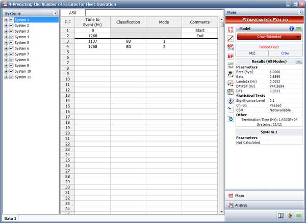
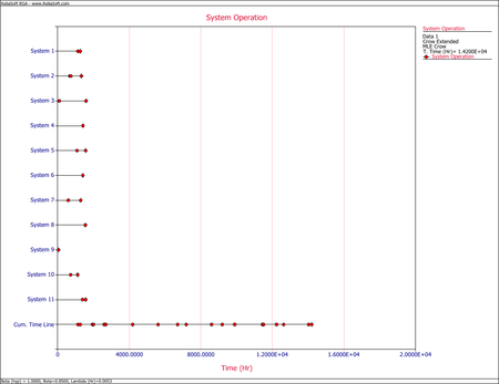
- Upon observing the estimated parameter [math]\displaystyle{ \beta \,\! }[/math], it does appear that the systems were randomly ordered since [math]\displaystyle{ \beta =0.8569\,\! }[/math]. This value is close to 1. You can also verify that the confidence bounds on [math]\displaystyle{ \beta \,\! }[/math] include 1 by going to the QCP and calculating the parameter bounds or by viewing the Beta Bounds plot. However, you can also determine graphically if the systems were randomly ordered by using the System Operation plot as shown below. Looking at the Cum. Time Line, it does not appear that the failures have a trend associated with them. Therefore, the systems can be assumed to be randomly ordered.
- After implementing the delayed fixes, the system's projected MTBF is equal to [math]\displaystyle{ 1035.6802\,\! }[/math] as shown in the plot below.
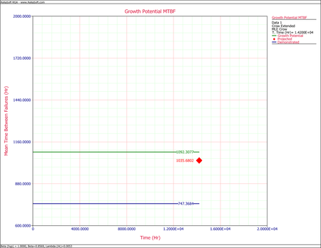
To estimate the number of failures during the next 4,000 hours, calculate the following:
[math]\displaystyle{ \begin{align} N=& \frac{4000}{1035.6802}\\ = & 3.8622\end{align}\,\! }[/math]
Therefore, it is estimated that [math]\displaystyle{ \approx\,\! }[/math] 4 failures will be observed during the next 4,000 hours of fleet operation.


General Examples
Example 5 (fleet data)
Eleven systems from the field were chosen for the purposes of a fleet analysis. Each system had at least one failure. All of the systems had a start time equal to zero and the last failure for each system corresponds to the end time. Group the data based on a fixed interval of 3000 hours and assume a fixed effectiveness factor equal to 0.4. Do the following:
1) Estimate the parameters of the Crow Extended model.
2) Based on the analysis does it appear that the systems were randomly ordered?
3) After the implementation of the delayed fixes, how many failures would you expect within the next 4000 hours of fleet operation.
| Table 13.9 - Fleet data for Example 5 | |
| System | Times-to-Failure |
|---|---|
| 1 | 1137 BD1, 1268 BD2 |
| 2 | 682 BD3, 744 A, 1336 BD1 |
| 3 | 95 BD1, 1593 BD3 |
| 4 | 1421 A |
| 5 | 1091 A, 1574 BD2 |
| 6 | 1415 BD4 |
| 7 | 598 BD4, 1290 BD1 |
| 8 | 1556 BD5 |
| 9 | 55 BD4 |
| 10 | 730 BD1, 1124 BD3 |
| 11 | 1400 BD4, 1568 A |
Solution to Example 5=
- 1) Figure Repair1 shows the estimated Crow Extended parameters.
- 2) Upon observing the estimated parameter [math]\displaystyle{ \beta }[/math] it does appear that the systems were randomly ordered since [math]\displaystyle{ \beta =0.8569 }[/math] . This value is close to 1. You can also verify that the confidence bounds on [math]\displaystyle{ \beta }[/math] include 1 by going to the QCP and calculating the parameter bounds or by viewing the Beta Bounds plot. However, you can also determine graphically if the systems were randomly ordered by using the System Operation plot as shown in Figure Repair2. Looking at the Cum. Time Line, it does not appear that the failures have a trend associated with them. Therefore, the systems can be assumed to be randomly ordered.
[math]\displaystyle{ }[/math]
Example 6 (repairable system data)
This case study is based on the data given in the article Graphical Analysis of Repair Data by Dr. Wayne Nelson [23]. The data in Table 13.10 represents repair data on an automatic transmission from a sample of 34 cars. For each car, the data set shows mileage at the time of each transmission repair, along with the latest mileage. The + indicates the latest mileage observed without failure. Car 1, for example, had a repair at 7068 miles and was observed until 26,744 miles. Do the following:
- 1) Estimate the parameters of the Power Law model.
- 2) Estimate the number of warranty claims for a 36,000 mile warranty policy for an estimated fleet of 35,000 vehicles.
| Table 13.10 - Automatic transmission data | ||||
| Car | Mileage | Car | Mileage | |
|---|---|---|---|---|
| 1 | 7068, 26744+ | 18 | 17955+ | |
| 2 | 28, 13809+ | 19 | 19507+ | |
| 3 | 48, 1440, 29834+ | 20 | 24177+ | |
| 4 | 530, 25660+ | 21 | 22854+ | |
| 5 | 21762+ | 22 | 17844+ | |
| 6 | 14235+ | 23 | 22637+ | |
| 7 | 1388, 18228+ | 24 | 375, 19607+ | |
| 8 | 21401+ | 25 | 19403+ | |
| 9 | 21876+ | 26 | 20997+ | |
| 10 | 5094, 18228+ | 27 | 19175+ | |
| 11 | 21691+ | 28 | 20425+ | |
| 12 | 20890+ | 29 | 22149+ | |
| 13 | 22486+ | 30 | 21144+ | |
| 14 | 19321+ | 31 | 21237+ | |
| 15 | 21585+ | 32 | 14281+ | |
| 16 | 18676+ | 33 | 8250, 21974+ | |
| 17 | 23520+ | 34 | 19250, 21888+ | |
Solution to Example 6
- 1) The estimated Power Law parameters are shown in Figure Repair3.
- 2) The expected number of failures at 36,000 miles can be estimated using the QCP as shown in Figure Repair4. The model predicts that 0.3559 failures per system will occur by 36,000 miles. This means that for a fleet of 35,000 vehicles, the expected warranty claims are 0.3559 * 35,000 = 12,456.
[math]\displaystyle{ }[/math]

[math]\displaystyle{ }[/math]

Example 7 (repairable system data)
Field data have been collected for a system that begins its wearout phase at time zero. The start time for each system is equal to zero and the end time for each system is 10,000 miles. Each system is scheduled to undergo an overhaul after a certain number of miles. It has been determined that the cost of an overhaul is four times more expensive than a repair. Table 13.11 presents the data. Do the following:
- 1) Estimate the parameters of the Power Law model.
- 2) Determine the optimum overhaul interval.
- 3) If [math]\displaystyle{ \beta \lt 1 }[/math] , would it be cost-effective to implement an overhaul policy?
| Table 13.11 - Field data | ||
| System 1 | System 2 | System 3 |
|---|---|---|
| 1006.3 | 722.7 | 619.1 |
| 2261.2 | 1950.9 | 1519.1 |
| 2367 | 3259.6 | 2956.6 |
| 2615.5 | 4733.9 | 3114.8 |
| 2848.1 | 5105.1 | 3657.9 |
| 4073 | 5624.1 | 4268.9 |
| 5708.1 | 5806.3 | 6690.2 |
| 6464.1 | 5855.6 | 6803.1 |
| 6519.7 | 6325.2 | 7323.9 |
| 6799.1 | 6999.4 | 7501.4 |
| 7342.9 | 7084.4 | 7641.2 |
| 7736 | 7105.9 | 7851.6 |
| 8246.1 | 7290.9 | 8147.6 |
| 7614.2 | 8221.9 | |
| 8332.1 | 9560.5 | |
| 8368.5 | 9575.4 | |
| 8947.9 | ||
| 9012.3 | ||
| 9135.9 | ||
| 9147.5 | ||
| 9601 | ||
Solution to Example 7
- 1) Figure Repair5 shows the estimated Power Law parameters.
- 2) The QCP can be used to calculate the optimum overhaul interval as shown in Figure Repair6.
- 3) Since [math]\displaystyle{ \beta \lt 1 }[/math] then the systems are not wearing out and it would not be cost-effective to implement an overhaul policy. An overhaul policy makes sense only if the systems are wearing out. Otherwise, an overhauled unit would have the same probability of failing as a unit that was not overhauled.
[math]\displaystyle{ }[/math]


Example 8 (repairable system data)
Failures and fixes of two repairable systems in the field are recorded. Both systems start from time 0. System 1 ends at time = 504 and system 2 ends at time = 541. All the BD modes are fixed at the end of the test. A fixed effectiveness factor equal to 0.6 is used. Answer the following questions:
- 1) Estimate the parameters of the Crow Extended model.
- 2) Calculate the projected MTBF after the delayed fixes.
- 3) What is the expected number of failures at time 1,000, if no fixes were performed for the future failures?
Solution to Example 8
- 1) Figure CrowExtendedRepair shows the estimated Crow Extended parameters.
- 2) Figure CrowExtendedMTBF shows the projected MTBF at time = 541 (i.e. the age of the oldest system).
- 3) Figure CrowExtendedNumofFailure shows the expected number of failures at time = 1,000.
[math]\displaystyle{ }[/math]


Fielded Systems
The previous chapters presented analysis methods for data obtained during developmental testing. However, data from systems in the field can also be analyzed in RGA. This type of data is called fielded systems data and is analogous to warranty data. Fielded systems can be categorized into two basic types: one-time or nonrepairable systems and reusable or repairable systems. In the latter case, under continuous operation, the system is repaired, but not replaced after each failure. For example, if a water pump in a vehicle fails, the water pump is replaced and the vehicle is repaired. Two types of analysis are presented in this chapter. The first is repairable systems analysis where the reliability of a system can be tracked and quantified based on data from multiple systems in the field. The second is fleet analysis where data from multiple systems in the field can be collected and analyzed so that reliability metrics for the fleet as a whole can be quantified. Template loop detected: Template:Repairable systems analysis rga
Template loop detected: Template:Parameter estimation fielded rga
Fleet analysis is similar to the repairable systems analysis described in the previous chapter. The main difference is that a fleet of systems is considered and the models are applied to the fleet failures rather than to the system failures. In other words, repairable system analysis models the number of system failures versus system time, whereas fleet analysis models the number of fleet failures versus fleet time.
The main motivation for fleet analysis is to enable the application of the Crow Extended model for fielded data. In many cases, reliability improvements might be necessary on systems that are already in the field. These types of reliability improvements are essentially delayed fixes (BD modes) as described in the Crow Extended chapter.
Introduction
Recall from the previous chapter that in order to make projections using the Crow Extended model, the [math]\displaystyle{ \beta \,\! }[/math] of the combined A and BD modes should be equal to 1. Since the failure intensity in a fielded system might be changing over time (e.g., increasing if the system wears out), this assumption might be violated. In such a scenario, the Crow Extended model cannot be used. However, if a fleet of systems is considered and the number of fleet failures versus fleet time is modeled, the failures might become random. This is because there is a mixture of systems within a fleet, new and old, and when the failures of this mixture of systems are viewed from a cumulative fleet time point of view, they may be random. The next two figures illustrate this concept. The first picture shows the number of failures over system age. It can be clearly seen that as the systems age, the intensity of the failures increases (wearout). The superposition system line, which brings the failures from the different systems under a single timeline, also illustrates this observation. On the other hand, if you take the same four systems and combine their failures from a fleet perspective, and consider fleet failures over cumulative fleet hours, then the failures seem to be random. The second picture illustrates this concept in the System Operation plot when you consider the Cum. Time Line. In this case, the [math]\displaystyle{ \beta \,\! }[/math] of the fleet will be equal to 1 and the Crow Extended model can be used for quantifying the effects of future reliability improvements on the fleet.
Methodology
The figures above illustrate that the difference between repairable system data analysis and fleet analysis is the way that the data set is treated. In fleet analysis, the time-to-failure data from each system is stacked to a cumulative timeline. For example, consider the two systems in the following table.
| System Data | ||
| System | Failure Times (hr) | End Time (hr) |
|---|---|---|
| 1 | 3, 7 | 10 |
| 2 | 4, 9, 13 | 15 |
Convert to Accumulated Timeline
The data set is first converted to an accumulated timeline, as follows:
- System 1 is considered first. The accumulated timeline is therefore 3 and 7 hours.
- System 1's end time is 10 hours. System 2's first failure is at 4 hours. This failure time is added to System 1's end time to give an accumulated failure time of 14 hours.
- The second failure for System 2 occurred 5 hours after the first failure. This time interval is added to the accumulated timeline to give 19 hours.
- The third failure for System 2 occurred 4 hours after the second failure. The accumulated failure time is 19 + 4 = 23 hours.
- System 2's end time is 15 hours, or 2 hours after the last failure. The total accumulated operating time for the fleet is 25 hours (23 + 2 = 25).
In general, the accumulated operating time [math]\displaystyle{ {{Y}_{j}}\,\! }[/math] is calculated by:
- [math]\displaystyle{ {{Y}_{j}}={{X}_{i,q}}+\underset{q=1}{\overset{K-1}{\mathop \sum }}\,{{T}_{q}},\text{ }m=1,2,...,N\,\! }[/math]
where:
- [math]\displaystyle{ {{X}_{i,q}}\,\! }[/math] is the [math]\displaystyle{ {{i}^{th}}\,\! }[/math] failure of the [math]\displaystyle{ {{q}^{th}}\,\! }[/math] system
- [math]\displaystyle{ {{T}_{q}}\,\! }[/math] is the end time of the [math]\displaystyle{ {{q}^{th}}\,\! }[/math] system
- [math]\displaystyle{ K\,\! }[/math] is the total number of systems
- [math]\displaystyle{ N\,\! }[/math] is the total number of failures from all systems ( [math]\displaystyle{ N=\underset{j=1}{\overset{K}{\mathop{\sum }}}\,{{N}_{q}}\,\! }[/math] )
As this example demonstrates, the accumulated timeline is determined based on the order of the systems. So if you consider the data in the table by taking System 2 first, the accumulated timeline would be: 4, 9, 13, 18, 22, with an end time of 25. Therefore, the order in which the systems are considered is somewhat important. However, in the next step of the analysis, the data from the accumulated timeline will be grouped into time intervals, effectively eliminating the importance of the order of the systems. Keep in mind that this will NOT always be true. This is true only when the order of the systems was random to begin with. If there is some logic/pattern in the order of the systems, then it will remain even if the cumulative timeline is converted to grouped data. For example, consider a system that wears out with age. This means that more failures will be observed as this system ages and these failures will occur more frequently. Within a fleet of such systems, there will be new and old systems in operation. If the data set collected is considered from the newest to the oldest system, then even if the data points are grouped, the pattern of fewer failures at the beginning and more failures at later time intervals will still be present. If the objective of the analysis is to determine the difference between newer and older systems, then that order for the data will be acceptable. However, if the objective of the analysis is to determine the reliability of the fleet, then the systems should be randomly ordered.
Analyze the Grouped Data
Once the accumulated timeline has been generated, it is then converted into grouped data. To accomplish this, a group interval is required. The group interval length should be chosen so that it is representative of the data. Also note that the intervals do not have to be of equal length. Once the data points have been grouped, the parameters can be obtained using maximum likelihood estimation as described in the Crow-AMSAA (NHPP) chapter. The data from the table above can be grouped into 5 hour intervals. This interval length is sufficiently large to insure that there are failures within each interval. The grouped data set is given in the following table.
| Grouped Data | |
| Failures in Interval | Interval End Time |
|---|---|
| 1 | 5 |
| 1 | 10 |
| 1 | 15 |
| 1 | 20 |
| 1 | 25 |
The Crow-AMSAA model for grouped failure times is used for the data, and the parameters of the model are solved by satisfying the following maximum likelihood equations (See Crow-AMSAA (NHPP)):
- [math]\displaystyle{ \widehat{\lambda }=\frac{n}{T_{k}^{\widehat{\beta }}}\,\! }[/math]
- [math]\displaystyle{ \underset{i=1}{\overset{k}{\mathop \sum }}\,{{n}_{i}}\left[ \frac{T_{i}^{\widehat{\beta }}\ln {{T}_{i-1}}-T_{i-1}^{\widehat{\beta }}\ln {{T}_{i-1}}}{T_{i}^{\widehat{\beta }}-T_{i-1}^{\widehat{\beta }}}-\ln {{T}_{k}} \right]=0 }[/math]
Fleet Analysis Example
The following table presents data for a fleet of 27 systems. A cycle is a complete history from overhaul to overhaul. The failure history for the last completed cycle for each system is recorded. This is a random sample of data from the fleet. These systems are in the order in which they were selected. Suppose the intervals to group the current data are 10,000; 20,000; 30,000; 40,000 and the final interval is defined by the termination time. Conduct the fleet analysis.
| Sample Fleet Data | |||
| System | Cycle Time [math]\displaystyle{ {{T}_{j}}\,\! }[/math] | Number of failures [math]\displaystyle{ {{N}_{j}}\,\! }[/math] | Failure Time [math]\displaystyle{ {{X}_{ij}}\,\! }[/math] |
|---|---|---|---|
| 1 | 1396 | 1 | 1396 |
| 2 | 4497 | 1 | 4497 |
| 3 | 525 | 1 | 525 |
| 4 | 1232 | 1 | 1232 |
| 5 | 227 | 1 | 227 |
| 6 | 135 | 1 | 135 |
| 7 | 19 | 1 | 19 |
| 8 | 812 | 1 | 812 |
| 9 | 2024 | 1 | 2024 |
| 10 | 943 | 2 | 316, 943 |
| 11 | 60 | 1 | 60 |
| 12 | 4234 | 2 | 4233, 4234 |
| 13 | 2527 | 2 | 1877, 2527 |
| 14 | 2105 | 2 | 2074, 2105 |
| 15 | 5079 | 1 | 5079 |
| 16 | 577 | 2 | 546, 577 |
| 17 | 4085 | 2 | 453, 4085 |
| 18 | 1023 | 1 | 1023 |
| 19 | 161 | 1 | 161 |
| 20 | 4767 | 2 | 36, 4767 |
| 21 | 6228 | 3 | 3795, 4375, 6228 |
| 22 | 68 | 1 | 68 |
| 23 | 1830 | 1 | 1830 |
| 24 | 1241 | 1 | 1241 |
| 25 | 2573 | 2 | 871, 2573 |
| 26 | 3556 | 1 | 3556 |
| 27 | 186 | 1 | 186 |
| Total | 52110 | 37 | |
Solution
The sample fleet data set can be grouped into 10,000; 20,000; 30,000; 40,000 and 52,110 time intervals. The following table gives the grouped data.
| Grouped Data | |
| Time | Observed Failures |
|---|---|
| 10,000 | 8 |
| 20,000 | 16 |
| 30,000 | 22 |
| 40,000 | 27 |
| 52,110 | 37 |
Based on the above time intervals, the maximum likelihood estimates of [math]\displaystyle{ \widehat{\lambda }\,\! }[/math] and [math]\displaystyle{ \widehat{\beta }\,\! }[/math] for this data set are then given by:
- [math]\displaystyle{ \begin{matrix} \widehat{\lambda }=0.00147 \\ \widehat{\beta }=0.93328 \\ \end{matrix}\,\! }[/math]
The next figure shows the System Operation plot.
Applying the Crow Extended Model to Fleet Data
As it was mentioned previously, the main motivation of the fleet analysis is to apply the Crow Extended model for in-service reliability improvements. The methodology to be used is identical to the application of the Crow Extended model for Grouped Data described in a previous chapter. Consider the fleet data from the example above. In order to apply the Crow Extended model, put [math]\displaystyle{ N=37\,\! }[/math] failure times on a cumulative time scale over [math]\displaystyle{ (0,T)\,\! }[/math], where [math]\displaystyle{ T=52110\,\! }[/math]. In the example, each [math]\displaystyle{ {{T}_{i}}\,\! }[/math] corresponds to a failure time [math]\displaystyle{ {{X}_{ij}}\,\! }[/math]. This is often not the situation. However, in all cases the accumulated operating time [math]\displaystyle{ {{Y}_{q}}\,\! }[/math] at a failure time [math]\displaystyle{ {{X}_{ir}}\,\! }[/math] is:
- [math]\displaystyle{ \begin{align} {{Y}_{q}}= & {{X}_{i,r}}+\underset{j=1}{\overset{r-1}{\mathop \sum }}\,{{T}_{j}},\ \ \ q=1,2,\ldots ,N \\ N= & \underset{j=1}{\overset{K}{\mathop \sum }}\,{{N}_{j}} \end{align}\,\! }[/math]
And [math]\displaystyle{ q\,\! }[/math] indexes the successive order of the failures. Thus, in this example [math]\displaystyle{ N=37,\,{{Y}_{1}}=1396,\,{{Y}_{2}}=5893,\,{{Y}_{3}}=6418,\ldots ,{{Y}_{37}}=52110\,\! }[/math]. See the table below.
| Test-Find-Test Fleet Data | ||||||
| [math]\displaystyle{ q\,\! }[/math] | [math]\displaystyle{ {{Y}_{q}}\,\! }[/math] | Mode | [math]\displaystyle{ q\,\! }[/math] | [math]\displaystyle{ {{Y}_{q}}\,\! }[/math] | Mode | |
|---|---|---|---|---|---|---|
| 1 | 1396 | BD1 | 20 | 26361 | BD1 | |
| 2 | 5893 | BD2 | 21 | 26392 | A | |
| 3 | 6418 | A | 22 | 26845 | BD8 | |
| 4 | 7650 | BD3 | 23 | 30477 | BD1 | |
| 5 | 7877 | BD4 | 24 | 31500 | A | |
| 6 | 8012 | BD2 | 25 | 31661 | BD3 | |
| 7 | 8031 | BD2 | 26 | 31697 | BD2 | |
| 8 | 8843 | BD1 | 27 | 36428 | BD1 | |
| 9 | 10867 | BD1 | 28 | 40223 | BD1 | |
| 10 | 11183 | BD5 | 29 | 40803 | BD9 | |
| 11 | 11810 | A | 30 | 42656 | BD1 | |
| 12 | 11870 | BD1 | 31 | 42724 | BD10 | |
| 13 | 16139 | BD2 | 32 | 44554 | BD1 | |
| 14 | 16104 | BD6 | 33 | 45795 | BD11 | |
| 15 | 18178 | BD7 | 34 | 46666 | BD12 | |
| 16 | 18677 | BD2 | 35 | 48368 | BD1 | |
| 17 | 20751 | BD4 | 36 | 51924 | BD13 | |
| 18 | 20772 | BD2 | 37 | 52110 | BD2 | |
| 19 | 25815 | BD1 | ||||
Each system failure time in the table above corresponds to a problem and a cause (failure mode). The management strategy can be to not fix the failure mode (A mode) or to fix the failure mode with a delayed corrective action (BD mode). There are [math]\displaystyle{ {{N}_{A}}=4\,\! }[/math] failures due to A failure modes. There are [math]\displaystyle{ {{N}_{BD}}=33\,\! }[/math] total failures due to [math]\displaystyle{ M=13\,\! }[/math] distinct BD failure modes. Some of the distinct BD modes had repeats of the same problem. For example, mode BD1 had 12 occurrences of the same problem. Therefore, in this example, there are 13 distinct corrective actions corresponding to 13 distinct BD failure modes.
The objective of the Crow Extended model is to estimate the impact of the 13 distinct corrective actions.The analyst will choose an average effectiveness factor (EF) based on the proposed corrective actions and historical experience. Historical industry and government data supports a typical average effectiveness factor [math]\displaystyle{ \overline{d}=.70\,\! }[/math] for many systems. In this example, an average EF of [math]\displaystyle{ \bar{d}=0.4\,\! }[/math] was assumed in order to be conservative regarding the impact of the proposed corrective actions. Since there are no BC failure modes (corrective actions applied during the test), the projected failure intensity is:
- [math]\displaystyle{ \widehat{r}(T)=\left( \frac{{{N}_{A}}}{T}+\underset{i=1}{\overset{M}{\mathop \sum }}\,(1-{{d}_{i}})\frac{{{N}_{i}}}{T} \right)+\overline{d}h(T)\,\! }[/math]
The first term is estimated by:
- [math]\displaystyle{ {{\widehat{\lambda }}_{A}}=\frac{{{N}_{A}}}{T}=0.000077\,\! }[/math]
The second term is:
- [math]\displaystyle{ \underset{i=1}{\overset{M}{\mathop \sum }}\,(1-{{d}_{i}})\frac{{{N}_{i}}}{T}=0.00038\,\! }[/math]
This estimates the growth potential failure intensity:
- [math]\displaystyle{ \begin{align} {{\widehat{\gamma }}_{GP}}(T)= & \frac{{{N}_{A}}}{T}+\underset{i=1}{\overset{M}{\mathop \sum }}\,(1-{{d}_{i}})\frac{{{N}_{i}}}{T} \\ = & 0.00046 \end{align}\,\! }[/math]
To estimate the last term [math]\displaystyle{ \overline{d}h(T)\,\! }[/math] of the Crow Extended model, partition the data in the table into intervals. This partition consists of [math]\displaystyle{ D\,\! }[/math] successive intervals. The length of the [math]\displaystyle{ {{q}^{th}}\,\! }[/math] interval is [math]\displaystyle{ {{L}_{q}},\,\! }[/math] [math]\displaystyle{ \,q=1,2,\ldots ,D\,\! }[/math]. It is not required that the intervals be of the same length, but there should be several (e.g., at least 5) cycles per interval on average. Also, let [math]\displaystyle{ {{S}_{1}}={{L}_{1}},\,\! }[/math] [math]\displaystyle{ {{S}_{2}}={{L}_{1}}+{{L}_{2}},\ldots ,\,\! }[/math] etc. be the accumulated time through the [math]\displaystyle{ {{q}^{th}}\,\! }[/math] interval. For the [math]\displaystyle{ {{q}^{th}}\,\! }[/math] interval, note the number of distinct BD modes, [math]\displaystyle{ M{{I}_{q}}\,\! }[/math], appearing for the first time, [math]\displaystyle{ q=1,2,\ldots ,D\,\! }[/math]. See the following table.
| Grouped Data for Distinct BD Modes | |||
| Interval | No. of Distinct BD Mode Failures | Length | Accumulated Time |
|---|---|---|---|
| 1 | [math]\displaystyle{ \text{MI}_{1}\,\! }[/math] | [math]\displaystyle{ \text{L}_{1}\,\! }[/math] | [math]\displaystyle{ \text{S}_{1}\,\! }[/math] |
| 2 | [math]\displaystyle{ \text{MI}_{2}\,\! }[/math] | [math]\displaystyle{ \text{L}_{2}\,\! }[/math] | [math]\displaystyle{ \text{S}_{2}\,\! }[/math] |
| . | . | . | . |
| . | . | . | . |
| . | . | . | . |
| D | [math]\displaystyle{ \text{MI}_{D}\,\! }[/math] | [math]\displaystyle{ \text{L}_{D}\,\! }[/math] | [math]\displaystyle{ \text{S}_{D}\,\! }[/math] |
The term [math]\displaystyle{ \widehat{h}(T)\,\! }[/math] is calculated as [math]\displaystyle{ \widehat{h}(T)=\widehat{\lambda }\widehat{\beta }{{T}^{\widehat{\beta }-1}}\,\! }[/math] and the values [math]\displaystyle{ \widehat{\lambda }\,\! }[/math] and [math]\displaystyle{ \widehat{\beta }\,\! }[/math] satisfy the maximum likelihood equations for grouped data (given in the Methodology section). This is the grouped data version of the Crow-AMSAA model applied only to the first occurrence of distinct BD modes.
For the data in the first table, the first 4 intervals had a length of 10,000 and the last interval was 12,110. Therefore, [math]\displaystyle{ D=5\,\! }[/math]. This choice gives an average of about 5 overhaul cycles per interval. See the table below.
| Grouped Data for Distinct BD Modes from Data in "Applying the Crow Extended Model to Fleet Data" | |||
| Interval | No. of Distinct BD Mode Failures | Length | Accumulated Time |
|---|---|---|---|
| 1 | 4 | 10000 | 10000 |
| 2 | 3 | 10000 | 20000 |
| 3 | 1 | 10000 | 30000 |
| 4 | 0 | 10000 | 40000 |
| 5 | 5 | 12110 | 52110 |
| Total | 13 | ||
Thus:
- [math]\displaystyle{ \begin{align} \widehat{\lambda }= & 0.00330 \\ \widehat{\beta }= & 0.76219 \end{align}\,\! }[/math]
This gives:
- [math]\displaystyle{ \begin{align} \widehat{h}(T)= & \widehat{\lambda }\widehat{\beta }{{T}^{\widehat{\beta }-1}} \\ = & 0.00019 \end{align}\,\! }[/math]
Consequently, for [math]\displaystyle{ \overline{d}=0.4\,\! }[/math] the last term of the Crow Extended model is given by:
- [math]\displaystyle{ \overline{d}h(T)=0.000076\,\! }[/math]
The projected failure intensity is:
- [math]\displaystyle{ \begin{align} \widehat{r}(T)= & \frac{{{N}_{A}}}{T}+\underset{i=1}{\overset{M}{\mathop \sum }}\,(1-{{d}_{i}})\frac{{{N}_{i}}}{T}+\overline{d}h(T) \\ = & 0.000077+0.6\times (0.00063)+0.4\times (0.00019) \\ = & 0.000533 \end{align}\,\! }[/math]
This estimates that the 13 proposed corrective actions will reduce the number of failures per cycle of operation hours from the current [math]\displaystyle{ \widehat{r}(0)=\tfrac{{{N}_{A}}+{{N}_{BD}}}{T}=0.00071\,\! }[/math] to [math]\displaystyle{ \widehat{r}(T)=0.00053.\,\! }[/math] The average time between failures is estimated to increase from the current 1408.38 hours to 1876.93 hours.
Confidence Bounds
For fleet data analysis using the Crow-AMSAA model, the confidence bounds are calculated using the same procedure described for the Crow-AMSAA (NHPP) model (See Crow-AMSAA Confidence Bounds). For fleet data analysis using the Crow Extended model, the confidence bounds are calculated using the same procedure described for the Crow Extended model (See Crow Extended Confidence Bounds).
More Examples
Predicting the Number of Failures for Fleet Operation
11 systems from the field were chosen for fleet analysis. Each system had at least one failure. All of the systems had a start time equal to zero and the last failure for each system corresponds to the end time. Group the data based on a fixed interval of 3,000 hours, and assume a fixed effectiveness factor equal to 0.4. Do the following:
- Estimate the parameters of the Crow Extended model.
- Based on the analysis, does it appear that the systems were randomly ordered?
- After the implementation of the delayed fixes, how many failures would you expect within the next 4,000 hours of fleet operation.
| Fleet Data | |
| System | Times-to-Failure |
|---|---|
| 1 | 1137 BD1, 1268 BD2 |
| 2 | 682 BD3, 744 A, 1336 BD1 |
| 3 | 95 BD1, 1593 BD3 |
| 4 | 1421 A |
| 5 | 1091 A, 1574 BD2 |
| 6 | 1415 BD4 |
| 7 | 598 BD4, 1290 BD1 |
| 8 | 1556 BD5 |
| 9 | 55 BD4 |
| 10 | 730 BD1, 1124 BD3 |
| 11 | 1400 BD4, 1568 A |
Solution
- The next figure shows the estimated Crow Extended parameters.
- Upon observing the estimated parameter [math]\displaystyle{ \beta \,\! }[/math], it does appear that the systems were randomly ordered since [math]\displaystyle{ \beta =0.8569\,\! }[/math]. This value is close to 1. You can also verify that the confidence bounds on [math]\displaystyle{ \beta \,\! }[/math] include 1 by going to the QCP and calculating the parameter bounds or by viewing the Beta Bounds plot. However, you can also determine graphically if the systems were randomly ordered by using the System Operation plot as shown below. Looking at the Cum. Time Line, it does not appear that the failures have a trend associated with them. Therefore, the systems can be assumed to be randomly ordered.
- After implementing the delayed fixes, the system's projected MTBF is equal to [math]\displaystyle{ 1035.6802\,\! }[/math] as shown in the plot below.
To estimate the number of failures during the next 4,000 hours, calculate the following:
[math]\displaystyle{ \begin{align} N=& \frac{4000}{1035.6802}\\ = & 3.8622\end{align}\,\! }[/math]
Therefore, it is estimated that [math]\displaystyle{ \approx\,\! }[/math] 4 failures will be observed during the next 4,000 hours of fleet operation.
General Examples
Example 5 (fleet data)
Eleven systems from the field were chosen for the purposes of a fleet analysis. Each system had at least one failure. All of the systems had a start time equal to zero and the last failure for each system corresponds to the end time. Group the data based on a fixed interval of 3000 hours and assume a fixed effectiveness factor equal to 0.4. Do the following:
1) Estimate the parameters of the Crow Extended model.
2) Based on the analysis does it appear that the systems were randomly ordered?
3) After the implementation of the delayed fixes, how many failures would you expect within the next 4000 hours of fleet operation.
| Table 13.9 - Fleet data for Example 5 | |
| System | Times-to-Failure |
|---|---|
| 1 | 1137 BD1, 1268 BD2 |
| 2 | 682 BD3, 744 A, 1336 BD1 |
| 3 | 95 BD1, 1593 BD3 |
| 4 | 1421 A |
| 5 | 1091 A, 1574 BD2 |
| 6 | 1415 BD4 |
| 7 | 598 BD4, 1290 BD1 |
| 8 | 1556 BD5 |
| 9 | 55 BD4 |
| 10 | 730 BD1, 1124 BD3 |
| 11 | 1400 BD4, 1568 A |
Solution to Example 5=
- 1) Figure Repair1 shows the estimated Crow Extended parameters.
- 2) Upon observing the estimated parameter [math]\displaystyle{ \beta }[/math] it does appear that the systems were randomly ordered since [math]\displaystyle{ \beta =0.8569 }[/math] . This value is close to 1. You can also verify that the confidence bounds on [math]\displaystyle{ \beta }[/math] include 1 by going to the QCP and calculating the parameter bounds or by viewing the Beta Bounds plot. However, you can also determine graphically if the systems were randomly ordered by using the System Operation plot as shown in Figure Repair2. Looking at the Cum. Time Line, it does not appear that the failures have a trend associated with them. Therefore, the systems can be assumed to be randomly ordered.
[math]\displaystyle{ }[/math]
Example 6 (repairable system data)
This case study is based on the data given in the article Graphical Analysis of Repair Data by Dr. Wayne Nelson [23]. The data in Table 13.10 represents repair data on an automatic transmission from a sample of 34 cars. For each car, the data set shows mileage at the time of each transmission repair, along with the latest mileage. The + indicates the latest mileage observed without failure. Car 1, for example, had a repair at 7068 miles and was observed until 26,744 miles. Do the following:
- 1) Estimate the parameters of the Power Law model.
- 2) Estimate the number of warranty claims for a 36,000 mile warranty policy for an estimated fleet of 35,000 vehicles.
| Table 13.10 - Automatic transmission data | ||||
| Car | Mileage | Car | Mileage | |
|---|---|---|---|---|
| 1 | 7068, 26744+ | 18 | 17955+ | |
| 2 | 28, 13809+ | 19 | 19507+ | |
| 3 | 48, 1440, 29834+ | 20 | 24177+ | |
| 4 | 530, 25660+ | 21 | 22854+ | |
| 5 | 21762+ | 22 | 17844+ | |
| 6 | 14235+ | 23 | 22637+ | |
| 7 | 1388, 18228+ | 24 | 375, 19607+ | |
| 8 | 21401+ | 25 | 19403+ | |
| 9 | 21876+ | 26 | 20997+ | |
| 10 | 5094, 18228+ | 27 | 19175+ | |
| 11 | 21691+ | 28 | 20425+ | |
| 12 | 20890+ | 29 | 22149+ | |
| 13 | 22486+ | 30 | 21144+ | |
| 14 | 19321+ | 31 | 21237+ | |
| 15 | 21585+ | 32 | 14281+ | |
| 16 | 18676+ | 33 | 8250, 21974+ | |
| 17 | 23520+ | 34 | 19250, 21888+ | |
Solution to Example 6
- 1) The estimated Power Law parameters are shown in Figure Repair3.
- 2) The expected number of failures at 36,000 miles can be estimated using the QCP as shown in Figure Repair4. The model predicts that 0.3559 failures per system will occur by 36,000 miles. This means that for a fleet of 35,000 vehicles, the expected warranty claims are 0.3559 * 35,000 = 12,456.
[math]\displaystyle{ }[/math]
[math]\displaystyle{ }[/math]
Example 7 (repairable system data)
Field data have been collected for a system that begins its wearout phase at time zero. The start time for each system is equal to zero and the end time for each system is 10,000 miles. Each system is scheduled to undergo an overhaul after a certain number of miles. It has been determined that the cost of an overhaul is four times more expensive than a repair. Table 13.11 presents the data. Do the following:
- 1) Estimate the parameters of the Power Law model.
- 2) Determine the optimum overhaul interval.
- 3) If [math]\displaystyle{ \beta \lt 1 }[/math] , would it be cost-effective to implement an overhaul policy?
| Table 13.11 - Field data | ||
| System 1 | System 2 | System 3 |
|---|---|---|
| 1006.3 | 722.7 | 619.1 |
| 2261.2 | 1950.9 | 1519.1 |
| 2367 | 3259.6 | 2956.6 |
| 2615.5 | 4733.9 | 3114.8 |
| 2848.1 | 5105.1 | 3657.9 |
| 4073 | 5624.1 | 4268.9 |
| 5708.1 | 5806.3 | 6690.2 |
| 6464.1 | 5855.6 | 6803.1 |
| 6519.7 | 6325.2 | 7323.9 |
| 6799.1 | 6999.4 | 7501.4 |
| 7342.9 | 7084.4 | 7641.2 |
| 7736 | 7105.9 | 7851.6 |
| 8246.1 | 7290.9 | 8147.6 |
| 7614.2 | 8221.9 | |
| 8332.1 | 9560.5 | |
| 8368.5 | 9575.4 | |
| 8947.9 | ||
| 9012.3 | ||
| 9135.9 | ||
| 9147.5 | ||
| 9601 | ||
Solution to Example 7
- 1) Figure Repair5 shows the estimated Power Law parameters.
- 2) The QCP can be used to calculate the optimum overhaul interval as shown in Figure Repair6.
- 3) Since [math]\displaystyle{ \beta \lt 1 }[/math] then the systems are not wearing out and it would not be cost-effective to implement an overhaul policy. An overhaul policy makes sense only if the systems are wearing out. Otherwise, an overhauled unit would have the same probability of failing as a unit that was not overhauled.
[math]\displaystyle{ }[/math]
Example 8 (repairable system data)
Failures and fixes of two repairable systems in the field are recorded. Both systems start from time 0. System 1 ends at time = 504 and system 2 ends at time = 541. All the BD modes are fixed at the end of the test. A fixed effectiveness factor equal to 0.6 is used. Answer the following questions:
- 1) Estimate the parameters of the Crow Extended model.
- 2) Calculate the projected MTBF after the delayed fixes.
- 3) What is the expected number of failures at time 1,000, if no fixes were performed for the future failures?
Solution to Example 8
- 1) Figure CrowExtendedRepair shows the estimated Crow Extended parameters.
- 2) Figure CrowExtendedMTBF shows the projected MTBF at time = 541 (i.e. the age of the oldest system).
- 3) Figure CrowExtendedNumofFailure shows the expected number of failures at time = 1,000.
[math]\displaystyle{ }[/math]