|
|
| (42 intermediate revisions by 8 users not shown) |
| Line 1: |
Line 1: |
| {{template:LDABOOK|5|Life Data Classifications}} | | <noinclude>{{template:LDABOOK|5|Life Data Classifications}}</noinclude> |
| | <!-- NOTE: THE SECTIONS THAT ARE WITHIN THE "INCLUDEONLY" TAGS APPLY ONLY TO ALTA AND APPEAR ONLY IN THE PAGE: Accelerated_Life_Testing_and_ALTA. |
| | THE ENTIRE ARTICLE, THAT INCLUDES BOTH THE WEIBULL++ AND ALTA CONTENT, APPEAR IN THE PAGE: Types_of_Life_Data.--> |
| | Statistical models rely extensively on data to make predictions. In life data analysis, the models are the ''statistical distributions'' and the data are the ''life data'' or ''times-to-failure data'' of our product. <includeonly>In the case of accelerated life data analysis, the models are the ''life-stress relationships'' and the data are the ''times-to-failure data at a specific stress level''.</includeonly>The accuracy of any prediction is directly proportional to the quality, accuracy and completeness of the supplied data. Good data, along with the appropriate model choice, usually results in good predictions. Bad or insufficient data will almost always result in bad predictions. |
|
| |
|
| ==Data & Data Types==
| | In the analysis of life data, we want to use all available data sets, which sometimes are incomplete or include uncertainty as to when a failure occurred. Life data can therefore be separated into two types: ''complete data'' (all information is available) or ''censored data'' (some of the information is missing). Each type is explained next. |
| Statistical models rely extensively on data to make predictions. In our case, the models are the ''statistical distributions'' and the data are the '' life data''or '' times-to-failure data'' of our product. The accuracy of any prediction is directly proportional to the quality, accuracy and completeness of the supplied data. Good data, along with the appropriate model choice, usually results in good predictions. Bad, or insufficient data, will almost always result in bad predictions.
| |
|
| |
|
| In the analysis of life data, we want to use all available data which sometimes is incomplete or includes uncertainty as to when a failure occurred. To accomplish this, we separate life data into two categories: complete (all information is available) or censored (some of the information is missing). This chapter details these data classification methods.
| | ==Complete Data== |
| ===Data Classification=== | |
| Most types of non-life data, as well as some life data, are what we term as ''complete data''. Complete data means that the value of each sample unit is observed or known. In many cases, life data contains uncertainty as to when exactly an event happened (''i.e.''when the unit failed). Data containing such uncertainty as to exactly when the event happened is termed as ''censored data''.
| |
| | |
| [[Image:ldachp4fig1.gif|thumb|center|300px|]]
| |
| | |
| | |
| ====Complete Data====
| |
| Complete data means that the value of each sample unit is observed or known. For example, if we had to compute the average test score for a sample of ten students, complete data would consist of the known score for each student. Likewise in the case of life data analysis, our data set (if complete) would be composed of the times-to-failure of all units in our sample. For example, if we tested five units and they all failed (and their times-to-failure were recorded), we would then have complete information as to the time of each failure in the sample. | | Complete data means that the value of each sample unit is observed or known. For example, if we had to compute the average test score for a sample of ten students, complete data would consist of the known score for each student. Likewise in the case of life data analysis, our data set (if complete) would be composed of the times-to-failure of all units in our sample. For example, if we tested five units and they all failed (and their times-to-failure were recorded), we would then have complete information as to the time of each failure in the sample. |
|
| |
|
| Complete data is much easier to work with than censored data. For example, it would be much harder to compute the average test score of the students if our data set were not complete, i.e.the average test score given scores of 30, 80, 60, 90, 95, three scores greater than 50, a score that is less than 70 and a score that is between 60 and 80.
| | [[Image:complete data.png|center|400px|]] |
| ====Censored Data ====
| |
| In many cases when life data are analyzed, all of the units in the sample may not have failed (i.e. the event of interest was not observed) or the exact times-to-failure of all the units are not known. This type of data is commonly called ''censored data''. There are three types of possible censoring schemes, right censored (also called suspended data), interval censored and left censored.
| |
| | |
| =====Right Censored (Suspended)=====
| |
| The most common case of censoring is what is referred to as ''right censored data'', or ''suspended data''. In the case of life data, these data sets are composed of units that did not fail. For example, if we tested five units and only three had failed by the end of the test, we would have suspended data (or right censored data) for the two unfailed units. The term ''right censored'' implies that the event of interest (i.e. the time-to-failure) is to the right of our data point. In other words, if the units were to keep on operating, the failure would occur at some time after our data point (or to the right on the time scale).
| |
| | |
| [[Image:ldachp4fig2.gif|thumb|center|300px|Graphical representation of right censored data.]] | |
| | |
| =====Interval Censored=====
| |
| The second type of censoring is commonly called ''interval censored data''. Interval censored data reflects uncertainty as to the exact times the units failed within an interval. This type of data frequently comes from tests or situations where the objects of interest are not constantly monitored. If we are running a test on five units and inspecting them every 100 hours, we only know that a unit failed or did not fail between inspections. More specifically, if we inspect a certain unit at 100 hours and find it is operating and then perform another inspection at 200 hours to find that the unit is no longer operating, we know that a failure occurred in the interval between 100 and 200 hours. In other words, the only information we have is that it failed in a certain interval of time. This is also called ''inspection data'' by some authors.
| |
| | |
| [[Image:ldachp4fig3.gif|thumb|center|300px|]]
| |
|
| |
|
| =====Left Censored===== | | ==Censored Data == |
| The third type of censoring is similar to the interval censoring and is called ''left censored data''. In left censored data, a failure time is only known to be before a certain time. For instance, we may know that a certain unit failed sometime before 100 hours but not exactly when. In other words, it could have failed any time between 0 and 100 hours. This is identical to ''interval censored data''in which the starting time for the interval is zero.
| | In many cases, all of the units in the sample may not have failed (i.e., the event of interest was not observed) or the exact times-to-failure of all the units are not known. This type of data is commonly called ''censored data''. There are three types of possible censoring schemes, right censored (also called suspended data), interval censored and left censored. |
|
| |
|
| | ===Right Censored (Suspension) Data=== |
| | The most common case of censoring is what is referred to as ''right censored data'', or ''suspended data''. In the case of life data, these data sets are composed of units that did not fail. For example, if we tested five units and only three had failed by the end of the test, we would have right censored data (or suspension data) for the two units that did not failed. The term ''right censored'' implies that the event of interest (i.e., the time-to-failure) is to the right of our data point. In other words, if the units were to keep on operating, the failure would occur at some time after our data point (or to the right on the time scale). |
|
| |
|
| [[Image:ldachp4fig4.gif|thumb|center|300px|]] | | [[Image:right censoring.png|center|400px|Graphical representation of right censored data.]] |
|
| |
|
| | ===Interval Censored Data=== |
| | The second type of censoring is commonly called ''interval censored data''. Interval censored data reflects uncertainty as to the exact times the units failed within an interval. This type of data frequently comes from tests or situations where the objects of interest are not constantly monitored. For example, if we are running a test on five units and inspecting them every 100 hours, we only know that a unit failed or did not fail between inspections. Specifically, if we inspect a certain unit at 100 hours and find it operating, and then perform another inspection at 200 hours to find that the unit is no longer operating, then the only information we have is that the unit failed at some point in the interval between 100 and 200 hours. This type of censored data is also called ''inspection data'' by some authors. |
|
| |
|
| ====Data Types and Weibull++====
| |
| Weibull++ allows you to use all of the above data types in a single data set. In other words, a data set can contain complete data, right censored data, interval censored data and left censored data. An overview of this is presented in this section.
| |
|
| |
|
| ====Grouped Data and Weibull++====
| | [[Image:interval censoring.png|center|400px|]] |
| All of the previously mentioned data types can also be put into groups. This is simply a way of collecting units with identical failure or censoring times. If ten units were put on test with the first four units failing at 10, 20, 30 and 40 hours respectively, and then the test were terminated after the fourth failure, you can group the last six units as a group of six suspensions at 40 hours. Weibull++ allows you to enter all types of data as groups, as shown in the following figure.
| |
|
| |
|
| [[Image:ldachp4fig5.gif|thumb|center|500px|]]
| |
|
| |
|
| Depending on the analysis method chosen, ''i.e.'' regression or maximum likelihood, Weibull++ treats grouped data differently. This was done by design to allow for more options and flexibility. Appendix B describes how Weibull++ treats grouped data.
| | It is generally recommended to avoid interval censored data because they are less informative compared to complete data. However, there are cases when interval data are unavoidable due to the nature of the product, the test and the test equipment. In those cases, caution must be taken to set the inspection intervals to be short enough to observe the spread of the failures. For example, if the inspection interval is too long, all the units in the test may fail within that interval, and thus no failure distribution could be obtained. |
|
| |
|
| ====Classifying Data in Weibull++====
| | <includeonly>In the case of accelerated life tests, the data set affects the accuracy of the fitted life-stress relationship, and subsequently, the extrapolation to Use Stress conditions. In this case, inspection intervals should be chosen according to the expected acceleration factor at each stress level, and therefore these intervals will be of different lengths for each stress level. |
| In Weibull++, data classifications are specified using data types. A single data set can contain any or all of the mentioned censoring schemes. Weibull++, through the use of the New Project Wizard and the New Data Sheet Wizard features, simplifies the choice of the appropriate data type for your data. Weibull++ uses the logic tree shown in Fig. 4-1 in deciding which is the appropriate data type for your data. | |
|
| |
|
| ===Analysis & Parameter Estimation Methods for Censored Data=== | | </includeonly>===Left Censored Data=== |
| In Chapter 3 we discussed parameter estimation methods for complete data. We will expand on that approach in this section by including estimation methods for the different types of censoring. The basic methods are still based on the same principles covered in Chapter 3, but modified to take into account the fact that some of the data points are censored. For example, assume that you were asked to find the mean (average) of 10, 20, a value that is between 25 and 40, a value that is greater than 30 and a value that is less than 50. In this case, the familiar method of determining the average is no longer applicable and special methods will need to be employed to handle the censored data in this data set.
| | The third type of censoring is similar to the interval censoring and is called ''left censored data''. In left censored data, a failure time is only known to be before a certain time. For instance, we may know that a certain unit failed sometime before 100 hours but not exactly when. In other words, it could have failed any time between 0 and 100 hours. This is identical to ''interval censored data'' in which the starting time for the interval is zero. |
|
| |
|
| [[Image:lda4.1.gif|thumb|center|600px|]]
| |
|
| |
|
| ==Analysis of Right Censored (Suspended) Data==
| | [[Image:left censoring.png|center|400px|]] |
| ====Background====
| |
|
| |
|
| All available data should be considered in the analysis of times-to-failure data. This includes the case when a particular unit in a sample has been removed from the test prior to failure. An item, or unit, which is removed from a reliability test prior to failure, or a unit which is in the field and is still operating at the time the reliability of these units is to be determined, is called a ''suspended item or ''right censored observation'' or '' right censored data point''. Suspended items analysis would also be considered when:
| | ===Grouped Data Analysis=== |
| #We need to make an analysis of the available results before test completion.
| | In the standard folio, data can be entered individually or in groups. Grouped data analysis is used for tests in which groups of units possess the same time-to-failure or in which groups of units were suspended at the same time. We highly recommend entering redundant data in groups. Grouped data speeds data entry by the user and significantly speeds up the calculations. |
| #The failure modes which are occurring are different than those anticipated and such units are withdrawn from the test.
| |
| #We need to analyze a single mode and the actual data set is comprised of multiple modes.
| |
| #A ''warranty analysis'' is to be made of all units in the field (non-failed and failed units). The non-failed units are considered to be suspended items (or right censored).
| |
|
| |
|
| ====Probability Plotting and Rank Regression Analysis of Right Censored Data====
| |
| When using the probability plotting or rank regression method to accommodate the fact that units in the data set did not fail, or were suspended, we need to adjust their probability of failure, or unreliability. As discussed in Chapter 3, estimates of the unreliability for complete data are obtained using the median ranks approach. The following methodology illustrates how adjusted median ranks are computed to account for right censored data.
| |
| To better illustrate the methodology, consider the following example [20] where five items are tested resulting in three failures and two suspensions.
| |
|
| |
|
| {|style= align="center" border="1"
| | ==A Note about Complete and Suspension Data== |
| !Item Number(Position)
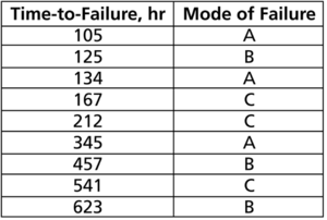
| | Depending on the event that we want to measure, data type classification (i.e., complete or suspension) can be open to interpretation. For example, under certain circumstances, and depending on the question one wishes to answer, a specimen that has failed might be classified as a suspension for analysis purposes. To illustrate this, consider the following times-to-failure data for a product that can fail due to modes A, B and C: |
| !State*"F" or "S"
| |
| !Life of item, hr
| |
| |-align="center"
| |
| |1||<math>F_1</math>||5,100
| |
| |-align="center"
| |
| |2||<math>S_1</math>||9,500
| |
| |-align="center"
| |
| |3||<math>F_2</math>||15,000
| |
| |-align="center"
| |
| |4||<math>S_2</math>||22,000
| |
| |-align="center"
| |
| |5||<math>F_3</math>||40,000
| |
| |}
| |
|
| |
|
|
| |
|
| | [[Image:time to failure chart.png|center|300px| ]] |
|
| |
|
| The methodology for plotting suspended items involves adjusting the rank positions and plotting the data based on new positions, determined by the location of the suspensions. If we consider these five units, the following methodology would be used:
| |
| The first item must be the first failure; hence, it is assigned failure order number <math>j=1</math>.
| |
| The actual failure order number (or position) of the second failure, <math>{{F}_{2}},</math> is in doubt. It could be either in position 2 or in position 3. Had <math>{{S}_{1}}</math> not been withdrawn from the test at 9,500 hours it could have operated successfully past 15,000 hours, thus placing <math>{{F}_{2}}</math> in position 2. Alternatively <math>{{S}_{1}}</math> could also have failed before 15,000 hours, thus placing <math>{{F}_{2}}</math> in position 3. In this case, the failure order number for <math>{{F}_{2}}</math> will be some number between 2 and 3. To determine this number, consider the following:
| |
|
| |
|
| We can find the number of ways the second failure can occur in either order number 2 (position 2) or order number 3 (position 3). The possible ways are listed next.
| | If the objective of the analysis is to determine the probability of failure of the product, regardless of the mode responsible for the failure, we would analyze the data with all data entries classified as failures (complete data). However, if the objective of the analysis is to determine the probability of failure of the product due to Mode A only, we would then choose to treat failures due to Modes B or C as suspension (right censored) data. Those data points would be treated as suspension data with respect to Mode A because the product operated until the recorded time without failure due to Mode A. |
|
| |
|
| | ==Fractional Failures== |
|
| |
|
| {|style= align="center" border="1"
| | After the completion of a reliability test or after failures are observed in the field, a redesign can be implemented to improve a product’s reliability. After the redesign, and before new failure data become available, it is often times desirable to “adjust” the reliability that was calculated from the previous design and take “credit” for this theoretical improvement. This can be achieved with fractional failures. Using past experience to estimate the effectiveness of a corrective action or redesign, an analysis can take credit for this improvement by adjusting the failure count. Therefore, if a corrective action on a failure mode is believed to be 70% effective, then the failure count can be reduced from 1 to 0.3 to reflect the effectiveness of the corrective action. |
| |-
| |
| |colspan="6" style="text-align:center;"|<math>F_2</math> in Position 2||rowspan="7" style="text=align:center;"|OR||colspan="2" style="text-align:center;"|<math>F_2</math> in Position 3
| |
| |-align="center"
| |
| |1||2||3||4||5||6 ||1||2
| |
| |-align="center"
| |
| |<math>F_1</math>||<math>F_1</math>||<math>F_1</math>||<math>F_1</math>||<math>F_1</math>||<math>F_1</math>|| <math>F_1</math> ||<math>F_1</math>
| |
| |-align="center"
| |
| |<math>F_2</math>||<math>F_2</math>||<math>F_2</math>||<math>F_2</math>||<math>F_2</math>||<math>F_2</math> ||<math>S_1</math>||<math>S_1</math>
| |
| |-align="center"
| |
| |<math>S_1</math>||<math>S_2</math>||<math>F_3</math>||<math>S_1</math>||<math>S_2</math>||<math>F_3</math> ||<math>F_2</math>||<math>F_2</math>
| |
| |-align="center"
| |
| |<math>S_2</math>||<math>S_1</math>||<math>S_1</math>||<math>F_3</math>||<math>F_3</math>||<math>S_2</math> ||<math>S_2</math>||<math>F_3</math>
| |
| |-align="center"
| |
| |<math>F_3</math>||<math>F_3</math>||<math>S_2</math>||<math>S_2</math>||<math>S_1</math>||<math>S_1</math> ||<math>F_3</math>||<math>S_2</math>
| |
| |}
| |
|
| |
|
| | For example, consider the following data set. |
|
| |
|
| | {| border="1" align="center" style="border-collapse: collapse;" cellpadding="5" cellspacing="5" |
| | |- align="center" |
| | !Number in State |
| | !State F or S |
| | !State End Time (Hr) |
| | |- align="center" |
| | |1 ||F || 105 |
| | |- align="center" |
| | |0.4 ||F || 168 |
| | |- align="center" |
| | |1 ||F || 220 |
| | |- align="center" |
| | |1 ||F || 290 |
| | |- align="center" |
| | |1 ||F || 410 |
| | |} |
|
| |
|
| It can be seen that <math>{{F}_{2}}</math> can occur in the second position six ways and in the third position two ways. The most probable position is the average of these possible ways, or the ''mean order number'' ( <math>MON</math> ), given by:
| | In this case, a design change has been implemented for the failure mode that occurred at 168 hours and is assumed to be 60% effective. In the background, Weibull++ converts this data set to: |
|
| |
|
| ::<math>{{F}_{2}}=MO{{N}_{2}}=\frac{(6\times 2)+(2\times 3)}{6+2}=2.25</math> | | {| border="1" align="center" style="border-collapse: collapse;" cellpadding="5" cellspacing="5" |
| | |- align="center" |
| | !Number in State |
| | !State F or S |
| | !State End Time (Hr) |
| | |- align="center" |
| | |1 ||F || 105 |
| | |- align="center" |
| | |0.4 ||F || 168 |
| | |- align="center" |
| | |0.6 ||S || 168 |
| | |- align="center" |
| | |1 ||F || 220 |
| | |- align="center" |
| | |1 ||F || 290 |
| | |- align="center" |
| | |1 ||F || 410 |
| | |} |
|
| |
|
| | If [[Parameter Estimation|Rank Regression]] is used to estimate distribution parameters, the median ranks for the previous data set are calculated as follows: |
|
| |
|
| Using the same logic on the third failure, it can be located in position numbers 3, 4 and 5 in the possible ways listed next.
| | {| border="1" align="center" style="border-collapse: collapse;" cellpadding="5" cellspacing="5" |
| | | |- align="center" |
| {|style= align="center" border="1" | | !Number in State |
| |-
| | !State F or S |
| |colspan="2" style="text-align:center;"|<math>F_3 \text{in Position 3}</math>|| rowspan="7" style="text-align:center;"|OR || colspan="3" style="text-align:center;"|<math>F_3 \text{in Position 4}</math> ||rowspan="7" style="text-align:center;"|OR||colspan="3" style="text-align:center;"|<math>F_3 \text{in Position 5}</math>
| | !State End Time (Hr) |
| |-
| |
| |1||2||1||2||3||1||2||3
| |
| |-
| |
| |<math>F_1</math>||<math>F_1</math>||<math>F_1</math>||<math>F_1</math>||<math>F_1</math>||<math>F_1</math>||<math>F_1</math>||<math>F_1</math>
| |
| |-
| |
| |<math>F_2</math>||<math>F_2</math>||<math>S_1</math>||<math>F_2</math>||<math>F_2</math>||<math>S_1</math>||<math>F_2</math>||<math>F_2</math>
| |
| |- | |
| |<math>F_3</math>||<math>F_3</math>||<math>F_2</math>||<math>S_1</math>||<math>S_2</math>||<math>F_2</math>||<math>S_1</math>||<math>S_2</math>
| |
| |-
| |
| |<math>S_1</math>||<math>S_2</math>||<math>F_3</math>||<math>F_3</math>||<math>F_3</math>||<math>S_2</math>||<math>S_2</math>||<math>S_1</math>
| |
| |-
| |
| |<math>S_2</math>||<math>S_1</math>||<math>S_2</math>||<math>S_2</math>||<math>S_1</math>||<math>F_3</math>||<math>F_3</math>||<math>F_3</math>
| |
| |}
| |
| | |
| | |
| Then, the mean order number for the third failure, (Item 5) is:
| |
| | |
| ::<math>MO{{N}_{3}}=\frac{(2\times 3)+(3\times 4)+(3\times 5)}{2+3+3}=4.125</math>
| |
| | |
| | |
| Once the mean order number for each failure has been established, we obtain the median rank positions for these failures at their mean order number. Specifically, we obtain the median rank of the order numbers 1, 2.25 and 4.125 out of a sample size of 5, as given next.
| |
| | |
| {|style= align="center" border="1"
| |
| |-
| |
| |colspan="3" style="text-align:center;"|Plotting Positions for the Failures(Sample Size=5)
| |
| |-align="center"
| |
| !Failure Number
| |
| !MON | | !MON |
| !Median Rank Position(%) | | !Median Rank (%) |
| |-align="center" | | |- align="center" |
| |1:<math>F_1</math>||1||13% | | |1 ||F || 105 || 1 ||12.945 |
| |-align="center" | | |- align="center" |
| |2:<math>F_2</math>||2.25||36% | | |0.4 ||F || 168 || 1.4 | 20.267 |
| |-align="center" | | |- align="center" |
| |3:<math>F_3</math>||4.125||71% | | |0.6 ||S || 168|| - || - |
| |} | | |- align="center" |
| | | |1 ||F || 220 || 2.55 || 41.616 |
| | | |- align="center" |
| Once the median rank values have been obtained, the probability plotting analysis is identical to that presented before. As you might have noticed, this methodology is rather laborious. Other techniques and shortcuts have been developed over the years to streamline this procedure. For more details on this method, see Kececioglu [20].
| | |1 ||F || 290 || 3.7 || 63.039 |
| | | |- align="center" |
| ====Shortfalls of this Rank Adjustment Method====
| | |1 ||F || 410 || 4.85 || 84.325 |
| Even though the rank adjustment method is the most widely used method for performing suspended items analysis, we would like to point out the following shortcoming.
| | |} |
| As you may have noticed from this analysis of suspended items, only the position where the failure occurred is taken into account, and not the exact time-to-suspension. For example, this methodology would yield the exact same results for the next two cases.
| |
| | |
| {|style= align="center" border="2"
| |
| |-
| |
| |colspan="3" style="text-align:center;"|Case 1 ||colspan="3" style="text-align:center;"|Case 2 | |
| |-align="center" | |
| !Item Number
| |
| !State*"F" or "S"
| |
| !Life of an item, hr
| |
| !Item number
| |
| !State*,"F" or "S"
| |
| !Life of item, hr
| |
| |-align="center" | |
| |1|| <math>F_1</math> ||1,000||1||<math>F_1</math>||1,000 | |
| |-align="center" | |
| |2||<math>S_1</math>||1,100||2||<math>S_1</math>||9,700 | |
| |-align="center" | |
| |3|| <math>S_2</math>||1,200||3||<math>S_2</math>||9,800 | |
| |-align="center" | |
| |4|| <math>S_3</math>||1,300||4||<math>S_3</math>||9,900 | |
| |-align="center"
| |
| |5|| <math>F_2</math>||10,000||5||<math>F_2</math>||10,000
| |
| |-align="center"
| |
| |colspan="3" style="text-align:center;"|<math>*F-Failed, S-Suspended</math>||colspan="3" style="text-align:center;"|<math>*F-Failed, S-Suspended</math>
| |
| |} | |
| | |
| | |
| This shortfall is significant when the number of failures is small and the number of suspensions is large and not spread uniformly between failures, as with these data. In cases like this, it is highly recommended that one use maximum likelihood estimation (MLE) to estimate the parameters instead of using least squares, since maximum likelihood does not look at ranks or plotting positions, but rather considers each unique time-to-failure or suspension.
| |
| For the data given above the results are as follows:
| |
| The estimated parameters using the method just described are the same for both cases (1 and 2):
| |
| | |
| ::<math>\begin{array}{*{35}{l}}
| |
| \widehat{\beta }= & \text{0}\text{.81} \\
| |
| \widehat{\eta }= & \text{11,417 hr} \\
| |
| \end{array}
| |
| </math>
| |
| | |
| However, the MLE results for Case 1 are:
| |
| | |
| ::<math>\begin{array}{*{35}{l}}
| |
| \widehat{\beta }= & \text{1}\text{.33} \\
| |
| \widehat{\eta }= & \text{6,900 hr} \\
| |
| \end{array}</math>
| |
| | |
| | |
| and the MLE results for Case 2 are:
| |
| | |
| As we can see, there is a sizable difference in the results of the two sets calculated using MLE and the results using regression. The results for both cases are identical when using the regression estimation technique, as regression considers only the positions of the suspensions. The MLE results are quite different for the two cases, with the second case having a much larger value of <math>\eta </math>, which is due to the higher values of the suspension times in Case 2. This is because the maximum likelihood technique, unlike rank regression, considers the values of the suspensions when estimating the parameters. This is illustrated in the following section.
| |
| | |
| ====MLE Analysis of Right Censored Data====
| |
| When performing maximum likelihood analysis on data with suspended items, the likelihood function needs to be expanded to take into account the suspended items. The overall estimation technique does not change, but another term is added to the likelihood function to account for the suspended items. Beyond that, the method of solving for the parameter estimates remains the same. For example, consider a distribution where <math>x</math> is a continuous random variable with <math>pdf</math> and <math>cdf</math>:
| |
| | |
| ::<math>\begin{align}
| |
| & f(x;{{\theta }_{1}},{{\theta }_{2}},...,{{\theta }_{k}}) \\
| |
| & F(x;{{\theta }_{1}},{{\theta }_{2}},...,{{\theta }_{k}})
| |
| \end{align}
| |
| </math>
| |
| | |
| where <math>{{\theta }_{1}},{{\theta }_{2}},...,{{\theta }_{k}}</math> are the unknown parameters which need to be estimated from <math>R</math> observed failures at <math>{{T}_{1}},{{T}_{2}}...{{T}_{R}},</math> and <math>M</math> observed suspensions at <math>{{S}_{1}},{{S}_{2}}</math> ... <math>{{S}_{M}},</math> then the likelihood function is formulated as follows:
| |
|
| |
|
| ::<math>\begin{align}
| |
| L({{\theta }_{1}},...,{{\theta }_{k}}|{{T}_{1}},...,{{T}_{R,}}{{S}_{1}},...,{{S}_{M}})= & \underset{i=1}{\overset{R}{\mathop \prod }}\,f({{T}_{i}};{{\theta }_{1}},{{\theta }_{2}},...,{{\theta }_{k}}) \\
| |
| & \cdot \underset{j=1}{\overset{M}{\mathop \prod }}\,[1-F({{S}_{j}};{{\theta }_{1}},{{\theta }_{2}},...,{{\theta }_{k}})]
| |
| \end{align}</math>
| |
|
| |
|
| The parameters are solved by maximizing this equation, as described in Chapter 3.
| | Given this information, the standard Rank Regression procedure is then followed to estimate parameters. |
| In most cases, no closed-form solution exists for this maximum or for the parameters. Solutions specific to each distribution utilizing MLE are presented in Appendix C.
| |
|
| |
|
| ====MLE Analysis of Interval and Left Censored Data====
| | If [[Maximum Likelihood Estimation|Maximum Likelihood Estimation (MLE)]] is used to estimate distribution parameters, the grouped data likelihood function is used with the number in group being a non-integer value. |
| The inclusion of left and interval censored data in an MLE solution for parameter estimates involves adding a term to the likelihood equation to account for the data types in question. When using interval data, it is assumed that the failures occurred in an interval, '' i.e.'' in the interval from time <math>A</math> to time <math>B</math> (or from time <math>0</math> to time <math>B</math> if left censored), where <math>A<B</math>.
| |
| In the case of interval data, and given <math>P</math> interval observations, the likelihood function is modified by multiplying the likelihood function with an additional term as follows:
| |
|
| |
|
| ::<math>\begin{align}
| |
| L({{\theta }_{1}},{{\theta }_{2}},...,{{\theta }_{k}}|{{x}_{1}},{{x}_{2}},...,{{x}_{P}})= & \underset{i=1}{\overset{P}{\mathop \prod }}\,\{F({{x}_{i}};{{\theta }_{1}},{{\theta }_{2}},...,{{\theta }_{k}}) \\
| |
| & \ \ -F({{x}_{i-1}};{{\theta }_{1}},{{\theta }_{2}},...,{{\theta }_{k}})\}
| |
| \end{align}
| |
| </math>
| |
|
| |
|
| Note that if only interval data are present, this term will represent the entire likelihood function for the MLE solution. The next section gives a formulation of the complete likelihood function for all possible censoring schemes.
| | ===Example=== |
|
| |
|
| ====ReliaSoft's Alternate Rank Method (RRM)====
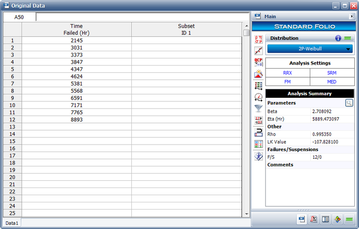
| | A component underwent a reliability test. 12 samples were run to failure. The following figure shows the failures and the analysis in a Weibull++ standard folio. |
| Difficulties arise when attempting the probability plotting or rank regression analysis of interval or left censored data, especially when an overlap on the intervals is present. This difficulty arises when attempting to estimate the exact time within the interval when the failure actually occurs. The ''standard regression method'' (SRM) is not applicable when dealing with interval data; thus ReliaSoft has formulated a more sophisticated methodology to allow for more accurate probability plotting and regression analysis of data sets with interval or left censored data. This method utilizes the traditional rank regression method and iteratively improves upon the computed ranks by parametrically recomputing new ranks and the most probable failure time for interval data. See Appendix B for a step-by-step example of this method.
| |
|
| |
|
| ====The Complete Likelihood Function====
| | [[Image:Fractional Failures 1.png|center|700px| ]] |
| We have now seen that obtaining MLE parameter estimates for different types of data involves incorporating different terms in the likelihood function to account for complete data, right censored data, and left, interval censored data. After including the terms for the different types of data, the likelihood function can now be expressed in its complete form or,
| |
|
| |
|
| ::<math>\begin{array}{*{35}{l}}
| |
| L= & \underset{i=1}{\mathop{\overset{R}{\mathop{\prod }}\,}}\,f({{T}_{i}};{{\theta }_{1}},...,{{\theta }_{k}})\cdot \underset{j=1}{\mathop{\overset{M}{\mathop{\prod }}\,}}\,[1-F({{S}_{j}};{{\theta }_{1}},...,{{\theta }_{k}})] \\
| |
| & \cdot \underset{l=1}{\mathop{\overset{P}{\mathop{\prod }}\,}}\,\left\{ F({{I}_{{{l}_{U}}}};{{\theta }_{1}},...,{{\theta }_{k}})-F({{I}_{{{l}_{L}}}};{{\theta }_{1}},...,{{\theta }_{k}}) \right\} \\
| |
| \end{array}
| |
| </math>
| |
|
| |
|
| :where
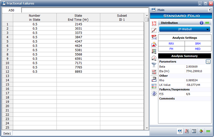
| | The analysts believe that the planned design improvements will yield 50% effectiveness. To estimate the reliability of the product based on the assumptions about the repair effectiveness, they enter the data in groups, counting a 0.5 failure for each group. The following figure shows the adjusted data set and the calculated parameters. |
|
| |
|
| ::<math> L\to L({{\theta }_{1}},...,{{\theta }_{k}}|{{T}_{1}},...,{{T}_{R}},{{S}_{1}},...,{{S}_{M}},{{I}_{1}},...{{I}_{P}}),</math> | | [[Image:Fractional Failures 2.png|center|700px| ]] |
|
| |
|
| :and
| |
| :# <math>R</math> is the number of units with exact failures
| |
| :# <math>M</math> is the number of suspended units
| |
| :# <math>P</math> is the number of units with left censored or interval times-to-failure
| |
| :# <math>{{\theta }_{k}}</math> are the parameters of the distribution
| |
| :# <math>{{T}_{i}}</math> is the <math>{{i}^{th}}</math> time to failure
| |
| :# <math>{{S}_{j}}</math> is the <math>{{j}^{th}}</math> time of suspension
| |
| :# <math>{{I}_{{{l}_{U}}}}</math> is the ending of the time interval of the <math>{{l}^{th}}</math> group
| |
| :# <math>{{I}_{{{l}_{L}}}}</math> is the beginning of the time interval of the <math>{l^{th}}</math> group
| |
|
| |
|
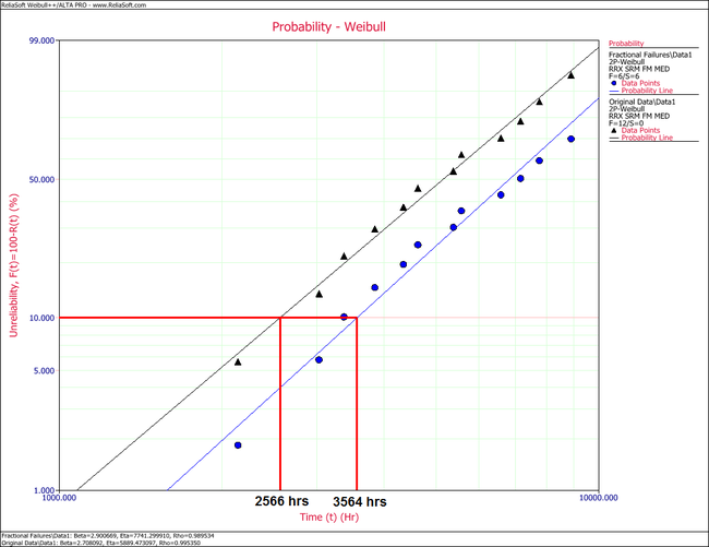
| | The following overlay plot of unreliability vs. time shows that by using fractional failures the estimated unreliability of the component has decreased, while the B10 life has increased from 2,566 hours to 3,564 hours. |
|
| |
|
| The total number of units is <math>N=R+M+P</math>. It should be noted that in this formulation if either <math>R</math>, <math>M</math> or <math>P</math> is zero the product term associated with them is assumed to be one and not zero.
| | [[Image:Fractional Failures 4.png|center|650px| ]] |
New format available! This reference is now available in a new format that offers faster page load, improved display for calculations and images, more targeted search and the latest content available as a PDF. As of September 2023, this Reliawiki page will not continue to be updated. Please update all links and bookmarks to the latest reference at help.reliasoft.com/reference/life_data_analysis
|
Chapter 5: Life Data Classification
|
Statistical models rely extensively on data to make predictions. In life data analysis, the models are the statistical distributions and the data are the life data or times-to-failure data of our product. The accuracy of any prediction is directly proportional to the quality, accuracy and completeness of the supplied data. Good data, along with the appropriate model choice, usually results in good predictions. Bad or insufficient data will almost always result in bad predictions.
In the analysis of life data, we want to use all available data sets, which sometimes are incomplete or include uncertainty as to when a failure occurred. Life data can therefore be separated into two types: complete data (all information is available) or censored data (some of the information is missing). Each type is explained next.
Complete Data
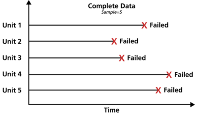
Complete data means that the value of each sample unit is observed or known. For example, if we had to compute the average test score for a sample of ten students, complete data would consist of the known score for each student. Likewise in the case of life data analysis, our data set (if complete) would be composed of the times-to-failure of all units in our sample. For example, if we tested five units and they all failed (and their times-to-failure were recorded), we would then have complete information as to the time of each failure in the sample.
Censored Data
In many cases, all of the units in the sample may not have failed (i.e., the event of interest was not observed) or the exact times-to-failure of all the units are not known. This type of data is commonly called censored data. There are three types of possible censoring schemes, right censored (also called suspended data), interval censored and left censored.
Right Censored (Suspension) Data
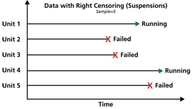
The most common case of censoring is what is referred to as right censored data, or suspended data. In the case of life data, these data sets are composed of units that did not fail. For example, if we tested five units and only three had failed by the end of the test, we would have right censored data (or suspension data) for the two units that did not failed. The term right censored implies that the event of interest (i.e., the time-to-failure) is to the right of our data point. In other words, if the units were to keep on operating, the failure would occur at some time after our data point (or to the right on the time scale).
Interval Censored Data
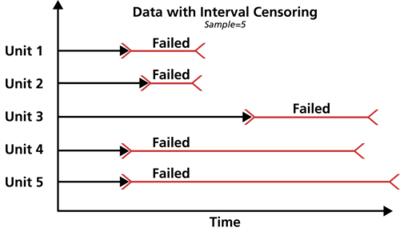
The second type of censoring is commonly called interval censored data. Interval censored data reflects uncertainty as to the exact times the units failed within an interval. This type of data frequently comes from tests or situations where the objects of interest are not constantly monitored. For example, if we are running a test on five units and inspecting them every 100 hours, we only know that a unit failed or did not fail between inspections. Specifically, if we inspect a certain unit at 100 hours and find it operating, and then perform another inspection at 200 hours to find that the unit is no longer operating, then the only information we have is that the unit failed at some point in the interval between 100 and 200 hours. This type of censored data is also called inspection data by some authors.
It is generally recommended to avoid interval censored data because they are less informative compared to complete data. However, there are cases when interval data are unavoidable due to the nature of the product, the test and the test equipment. In those cases, caution must be taken to set the inspection intervals to be short enough to observe the spread of the failures. For example, if the inspection interval is too long, all the units in the test may fail within that interval, and thus no failure distribution could be obtained.
Left Censored Data
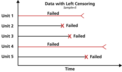
The third type of censoring is similar to the interval censoring and is called left censored data. In left censored data, a failure time is only known to be before a certain time. For instance, we may know that a certain unit failed sometime before 100 hours but not exactly when. In other words, it could have failed any time between 0 and 100 hours. This is identical to interval censored data in which the starting time for the interval is zero.
Grouped Data Analysis
In the standard folio, data can be entered individually or in groups. Grouped data analysis is used for tests in which groups of units possess the same time-to-failure or in which groups of units were suspended at the same time. We highly recommend entering redundant data in groups. Grouped data speeds data entry by the user and significantly speeds up the calculations.
A Note about Complete and Suspension Data
Depending on the event that we want to measure, data type classification (i.e., complete or suspension) can be open to interpretation. For example, under certain circumstances, and depending on the question one wishes to answer, a specimen that has failed might be classified as a suspension for analysis purposes. To illustrate this, consider the following times-to-failure data for a product that can fail due to modes A, B and C:
If the objective of the analysis is to determine the probability of failure of the product, regardless of the mode responsible for the failure, we would analyze the data with all data entries classified as failures (complete data). However, if the objective of the analysis is to determine the probability of failure of the product due to Mode A only, we would then choose to treat failures due to Modes B or C as suspension (right censored) data. Those data points would be treated as suspension data with respect to Mode A because the product operated until the recorded time without failure due to Mode A.
Fractional Failures
After the completion of a reliability test or after failures are observed in the field, a redesign can be implemented to improve a product’s reliability. After the redesign, and before new failure data become available, it is often times desirable to “adjust” the reliability that was calculated from the previous design and take “credit” for this theoretical improvement. This can be achieved with fractional failures. Using past experience to estimate the effectiveness of a corrective action or redesign, an analysis can take credit for this improvement by adjusting the failure count. Therefore, if a corrective action on a failure mode is believed to be 70% effective, then the failure count can be reduced from 1 to 0.3 to reflect the effectiveness of the corrective action.
For example, consider the following data set.
| Number in State
|
State F or S
|
State End Time (Hr)
|
| 1 |
F |
105
|
| 0.4 |
F |
168
|
| 1 |
F |
220
|
| 1 |
F |
290
|
| 1 |
F |
410
|
In this case, a design change has been implemented for the failure mode that occurred at 168 hours and is assumed to be 60% effective. In the background, Weibull++ converts this data set to:
| Number in State
|
State F or S
|
State End Time (Hr)
|
| 1 |
F |
105
|
| 0.4 |
F |
168
|
| 0.6 |
S |
168
|
| 1 |
F |
220
|
| 1 |
F |
290
|
| 1 |
F |
410
|
If Rank Regression is used to estimate distribution parameters, the median ranks for the previous data set are calculated as follows:
| Number in State
|
State F or S
|
State End Time (Hr)
|
MON
|
Median Rank (%)
|
| 1 |
F |
105 |
1 |
12.945
|
| 0.4 |
F |
168 |
20.267
|
| 0.6 |
S |
168 |
- |
-
|
| 1 |
F |
220 |
2.55 |
41.616
|
| 1 |
F |
290 |
3.7 |
63.039
|
| 1 |
F |
410 |
4.85 |
84.325
|
Given this information, the standard Rank Regression procedure is then followed to estimate parameters.
If Maximum Likelihood Estimation (MLE) is used to estimate distribution parameters, the grouped data likelihood function is used with the number in group being a non-integer value.
Example
A component underwent a reliability test. 12 samples were run to failure. The following figure shows the failures and the analysis in a Weibull++ standard folio.
The analysts believe that the planned design improvements will yield 50% effectiveness. To estimate the reliability of the product based on the assumptions about the repair effectiveness, they enter the data in groups, counting a 0.5 failure for each group. The following figure shows the adjusted data set and the calculated parameters.
The following overlay plot of unreliability vs. time shows that by using fractional failures the estimated unreliability of the component has decreased, while the B10 life has increased from 2,566 hours to 3,564 hours.

