Inverse Power Law Example: Difference between revisions
Jump to navigation
Jump to search
Kate Racaza (talk | contribs) m (moved Template:Example:IPL to Inverser Power Law Example: incorrect namespace) |
Kate Racaza (talk | contribs) (added link to ALTA book) |
||
| Line 1: | Line 1: | ||
<noinclude>{{Banner ALTA Examples}} | |||
''This example appears in the [[Inverse_Power_Law_(IPL)_Relationship#IPL-Weibull|Accelerated Life Testing Data Analysis Reference]] book.'' | |||
</noinclude> | |||
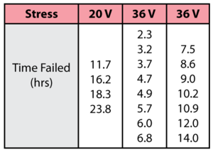
Consider the following times-to-failure data at two different stress levels. | Consider the following times-to-failure data at two different stress levels. | ||
[[Image:chp8ex1table.png|center|300px|''Pdf'' of the lognormal distribution with different log-std values.]] | [[Image:chp8ex1table.png|center|300px|''Pdf'' of the lognormal distribution with different log-std values.]] | ||
The data set was analyzed jointly | |||
The data set was analyzed jointly in an ALTA standard folio using the IPL-Weibull relationship model, with a complete MLE solution over the entire data set. The analysis yields: | |||
::<math>\widehat{\beta }=2.616464</math> | ::<math>\widehat{\beta }=2.616464</math> | ||
Revision as of 01:46, 14 August 2012
 |
New format available! This reference is now available in a new format that offers faster page load, improved display for calculations and images and more targeted search.
As of January 2024, this Reliawiki page will not continue to be updated. Please update all links and bookmarks to the latest references at ALTA examples and ALTA reference examples.
This example appears in the Accelerated Life Testing Data Analysis Reference book.
Consider the following times-to-failure data at two different stress levels.

The data set was analyzed jointly in an ALTA standard folio using the IPL-Weibull relationship model, with a complete MLE solution over the entire data set. The analysis yields:
- [math]\displaystyle{ \widehat{\beta }=2.616464 }[/math]
- [math]\displaystyle{ \widehat{K}=0.001022 }[/math]
- [math]\displaystyle{ \widehat{n}=1.327292 }[/math]