Inverse Power Law Example: Difference between revisions
Jump to navigation
Jump to search
Chris Kahn (talk | contribs) |
|||
| Line 1: | Line 1: | ||
===IPL-Weibull Example=== | ===IPL-Weibull Example=== | ||
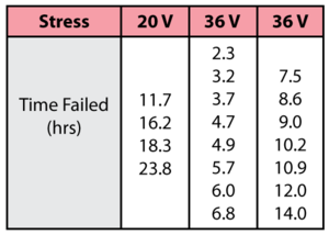
Consider the following times-to-failure data at two different stress levels. | Consider the following times-to-failure data at two different stress levels. | ||
[[Image:chp8ex1table.png|center|300px|''Pdf'' of the lognormal distribution with different log-std values.]] | [[Image:chp8ex1table.png|center|300px|''Pdf'' of the lognormal distribution with different log-std values.]] | ||
The data set was analyzed jointly and with a complete MLE solution over the entire data set using ReliaSoft's ALTA. The analysis yields: | The data set was analyzed jointly and with a complete MLE solution over the entire data set using ReliaSoft's ALTA. The analysis yields: | ||
::<math>\widehat{\beta }=2.616464</math> | ::<math>\widehat{\beta }=2.616464</math> | ||
::<math>\widehat{K}=0.001022</math> | ::<math>\widehat{K}=0.001022</math> | ||
::<math>\widehat{n}=1.327292</math> | ::<math>\widehat{n}=1.327292</math> | ||
Revision as of 02:02, 9 August 2012
IPL-Weibull Example
Consider the following times-to-failure data at two different stress levels.

The data set was analyzed jointly and with a complete MLE solution over the entire data set using ReliaSoft's ALTA. The analysis yields:
- [math]\displaystyle{ \widehat{\beta }=2.616464 }[/math]
- [math]\displaystyle{ \widehat{K}=0.001022 }[/math]
- [math]\displaystyle{ \widehat{n}=1.327292 }[/math]