Introduction to Life Data Analysis

Reliability Life Data Analysis refers to the study and modeling of observed product lives. Life data can be lifetimes of products in the marketplace, such as the time the product operated successfully or the time the product operated before it failed. These lifetimes can be measured in hours, miles, cycles-to-failure, stress cycles or any other metric with which the life or exposure of a product can be measured. All such data of product lifetimes can be encompassed in the term life data or, more specifically, product life data. The subsequent analysis and prediction are described as life data analysis. For the purpose of this reference, we will limit our examples and discussions to lifetimes of inanimate objects, such as equipment, components and systems as they apply to reliability engineering, however the same concepts can be applied in other areas.
An Overview of Basic Concepts
When performing life data analysis (also commonly referred to as Weibull analysis), the practitioner attempts to make predictions about the life of all products in the population by fitting a statistical distribution (model) to life data from a representative sample of units. The parameterized distribution for the data set can then be used to estimate important life characteristics of the product such as reliability or probability of failure at a specific time, the mean life and the failure rate. Life data analysis requires the practitioner to:
- Gather life data for the product.
- Select a lifetime distribution that will fit the data and model the life of the product.
- Estimate the parameters that will fit the distribution to the data.
- Generate plots and results that estimate the life characteristics of the product, such as the reliability or mean life.
Lifetime Distributions (Life Data Models)
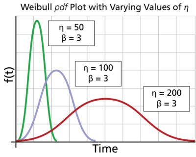
Statistical distributions have been formulated by statisticians, mathematicians and engineers to mathematically model or represent certain behavior. The probability density function (pdf) is a mathematical function that describes the distribution. The pdf can be represented mathematically or on a plot where the x-axis represents time, as shown next.
The 3-parameter Weibull pdf is given by:
- [math]\displaystyle{ f(t)={ \frac{\beta }{\eta }}\left( {\frac{t-\gamma }{\eta }}\right) ^{\beta -1}e^{-\left( {\frac{t-\gamma }{\eta }}\right) ^{\beta }} \,\! }[/math]
where:
- [math]\displaystyle{ f(t)\geq 0,\text{ }t\geq \gamma \,\! }[/math]
- [math]\displaystyle{ \beta\gt 0\ \,\! }[/math]
- [math]\displaystyle{ \eta \gt 0 \,\! }[/math]
- [math]\displaystyle{ -\infty \lt \gamma \lt +\infty \,\! }[/math]
and:
- [math]\displaystyle{ \eta= \,\! }[/math] scale parameter, or characteristic life
- [math]\displaystyle{ \beta= \,\! }[/math] shape parameter (or slope)
- [math]\displaystyle{ \gamma= \,\! }[/math] location parameter (or failure free life)
Some distributions, such as the Weibull and lognormal, tend to better represent life data and are commonly called "lifetime distributions" or "life distributions." In fact, life data analysis is sometimes called "Weibull analysis" because the Weibull distribution, formulated by Professor Waloddi Weibull, is a popular distribution for analyzing life data. The Weibull model can be applied in a variety of forms (including 1-parameter, 2-parameter, 3-parameter or mixed Weibull). Other commonly used life distributions include the exponential, lognormal and normal distributions. The analyst chooses the life distribution that is most appropriate to model each particular data set based on past experience and goodness-of-fit tests.
Parameter Estimation
In order to fit a statistical model to a life data set, the analyst estimates the parameters of the life distribution that will make the function most closely fit the data. The parameters control the scale, shape and location of the pdf function. For example, in the 3-parameter Weibull model (shown above), the scale parameter, [math]\displaystyle{ \eta\,\! }[/math], defines where the bulk of the distribution lies. The shape parameter, [math]\displaystyle{ \beta\,\! }[/math], defines the shape of the distribution and the location parameter, [math]\displaystyle{ \gamma\,\! }[/math], defines the location of the distribution in time.
Several methods have been devised to estimate the parameters that will fit a lifetime distribution to a particular data set. Some available parameter estimation methods include probability plotting, rank regression on x (RRX), rank regression on y (RRY) and maximum likelihood estimation (MLE). The appropriate analysis method will vary depending on the data set and, in some cases, on the life distribution selected.
Calculated Results and Plots
Once you have calculated the parameters to fit a life distribution to a particular data set, you can obtain a variety of plots and calculated results from the analysis, including:
- Reliability Given Time: The probability that a unit will operate successfully at a particular point in time. For example, there is an 88% chance that the product will operate successfully after 3 years of operation.
- Probability of Failure Given Time: The probability that a unit will be failed at a particular point in time. Probability of failure is also known as "unreliability" and it is the reciprocal of the reliability. For example, there is a 12% chance that the unit will be failed after 3 years of operation (probability of failure or unreliability) and an 88% chance that it will operate successfully (reliability).
- Mean Life: The average time that the units in the population are expected to operate before failure. This metric is often referred to as "mean time to failure" (MTTF) or "mean time before failure" (MTBF).
- Failure Rate: The number of failures per unit time that can be expected to occur for the product.
- Warranty Time: The estimated time when the reliability will be equal to a specified goal. For example, the estimated time of operation is 4 years for a reliability of 90%.
- B(X) Life: The estimated time when the probability of failure will reach a specified point (X%). For example, if 10% of the products are expected to fail by 4 years of operation, then the B(10) life is 4 years. (Note that this is equivalent to a warranty time of 4 years for a 90% reliability.)
- Probability Plot: A plot of the probability of failure over time. (Note that probability plots are based on the linearization of a specific distribution. Consequently, the form of a probability plot for one distribution will be different than the form for another. For example, an exponential distribution probability plot has different axes than those of a normal distribution probability plot.)
- Reliability vs. Time Plot: A plot of the reliability over time.
- pdf Plot: A plot of the probability density function (pdf).
- Failure Rate vs. Time Plot: A plot of the failure rate over time.
- Contour Plot: A graphical representation of the possible solutions to the likelihood ratio equation. This is employed to make comparisons between two different data sets.
Confidence Bounds
Because life data analysis results are estimates based on the observed lifetimes of a sampling of units, there is uncertainty in the results due to the limited sample sizes. "Confidence bounds" (also called "confidence intervals") are used to quantify this uncertainty due to sampling error by expressing the confidence that a specific interval contains the quantity of interest. Whether or not a specific interval contains the quantity of interest is unknown.
Confidence bounds can be expressed as two-sided or one-sided. Two-sided bounds are used to indicate that the quantity of interest is contained within the bounds with a specific confidence. One-sided bounds are used to indicate that the quantity of interest is above the lower bound or below the upper bound with a specific confidence. The appropriate type of bounds depends on the application. For example, the analyst would use a one-sided lower bound on reliability, a one-sided upper bound for percent failing under warranty and two-sided bounds on the parameters of the distribution. (Note that one-sided and two-sided bounds are related. For example, the 90% lower two-sided bound is the 95% lower one-sided bound and the 90% upper two-sided bounds is the 95% upper one-sided bound.)
Reliability Engineering
Since the beginning of history, humanity has attempted to predict the future. Watching the flight of birds, the movement of the leaves on the trees and other methods were some of the practices used. Fortunately, today's engineers do not have to depend on Pythia or a crystal ball in order to predict the future of their products. Through the use of life data analysis, reliability engineers use product life data to determine the probability and capability of parts, components, and systems to perform their required functions for desired periods of time without failure, in specified environments.

Life data can be lifetimes of products in the marketplace, such as the time the product operated successfully or the time the product operated before it failed. These lifetimes can be measured in hours, miles, cycles-to-failure, stress cycles or any other metric with which the life or exposure of a product can be measured. All such data of product lifetimes can be encompassed in the term life data or, more specifically, product life data. The subsequent analysis and prediction are described as life data analysis. For the purpose of this reference, we will limit our examples and discussions to lifetimes of inanimate objects, such as equipment, components and systems as they apply to reliability engineering. Before performing life data analysis, the failure mode and the life units (hours, cycles, miles, etc.) must be specified and clearly defined. Further, it is quite necessary to define exactly what constitutes a failure. In other words, before performing the analysis it must be clear when the product is considered to have actually failed. This may seem rather obvious, but it is not uncommon for problems with failure definitions or time unit discrepancies to completely invalidate the results of expensive and time consuming life testing and analysis.
Estimation
In life data analysis and reliability engineering, the output of the analysis is always an estimate. The true value of the probability of failure, the probability of success (or reliability ), the mean life, the parameters of a distribution or any other applicable parameter is never known, and will almost certainly remain unknown to us for all practical purposes. Granted, once a product is no longer manufactured and all units that were ever produced have failed and all of that data has been collected and analyzed, one could claim to have learned the true value of the reliability of the product. Obviously, this is not a common occurrence.
The objective of reliability engineering and life data analysis is to accurately estimate these true values. For example, let's assume that our job is to estimate the number of black marbles in a giant swimming pool filled with black and white marbles. One method is to pick out a small sample of marbles and count the black ones. Suppose we picked out ten marbles and counted four black marbles.

Based on this sampling, the estimate would be that 40% of the marbles are black. If we put the ten marbles back in the pool and repeated this step again, we might get five black marbles, changing the estimate to 50% black marbles. The range of our estimate for the percentage of black marbles in the pool is 40% to 50%. If we now repeat the experiment and pick out 1,000 marbles, we might get results for the number of black marbles such as 445 and 495 black marbles for each trial. In this case, we note that our estimate for the percentage of black marbles has a narrower range, or 44.5% to 49.5%. Using this, we can see that the larger the sample size, the narrower the estimate range and, presumably, the closer the estimate range is to the true value.
A Brief Introduction to Reliability
A Formal Definition
Reliability engineering provides the theoretical and practical tools whereby the probability and capability of parts, components, equipment, products and systems to perform their required functions for desired periods of time without failure, in specified environments and with a desired confidence, can be specified, designed in, predicted, tested and demonstrated, as discussed in Kececioglu [19].
Reliability Engineering and Business Plans
Reliability engineering assessment is based on the results of testing from in-house (or contracted) labs and data pertaining to the performance results of the product in the field. The data produced by these sources are utilized to accurately measure and improve the reliability of the products being produced. This is particularly important as market concerns drive a constant push for cost reduction. However, one must be able to keep a perspective on the big picture instead of merely looking for the quick fix. It is often the temptation to cut corners and save initial costs by using cheaper parts or cutting testing programs. Unfortunately, cheaper parts are usually less reliable and inadequate testing programs can allow products with undiscovered flaws to get out into the field. A quick savings in the short term by the use of cheaper components or small test sample sizes will usually result in higher long-term costs in the form of warranty costs or loss of customer confidence. The proper balance must be struck between reliability, customer satisfaction, time to market, sales and features. The figure below illustrates this concept. The polygon on the left represents a properly balanced project. The polygon on the right represents a project in which reliability and customer satisfaction have been sacrificed for the sake of sales and time to market.

Through proper testing and analysis in the in-house testing labs, as well as collection of adequate and meaningful data on a product's performance in the field, the reliability of any product can be measured, tracked and improved, leading to a balanced organization with a financially healthy outlook for the future.
Key Reasons for Reliability Engineering
- For a company to succeed in today's highly competitive and technologically complex environment, it is ‘‘essential‘‘ that it knows the reliability of its product and is able to control it in order to produce products at an optimum reliability level. This yields the minimum life-cycle cost for the user and minimizes the manufacturer's costs of such a product without compromising the product's reliability and quality, as discussed in Kececioglu [19].
- Our growing dependence on technology requires that the products that make up our daily lives successfully work for the desired or designed-in period of time. It is not sufficient that a product works for time shorter than its mission duration, but at the same time there is no need to design a product to operate much past its intended life, since this would impose additional costs on the manufacturer. In today's complex world where many important operations are performed with automated equipment, we are dependent on the successful operation of these equipment (i.e., their reliability) and, if they fail, on their quick restoration to function (i.e., their maintainability), as discussed in Kececioglu [19].
- Product failures have varying effects, ranging from those that cause minor nuisances, such as the failure of a television's remote control (which can become a major nuisance, if not a catastrophe, depending on the football schedule of the day), to catastrophic failures involving loss of life and property, such as an aircraft accident. Reliability engineering was born out of the necessity to avoid such catastrophic events and, with them, the unnecessary loss of life and property. It is not surprising that Boeing was one of the first commercial companies to embrace and implement reliability engineering, the success of which can be seen in the safety of today's commercial air travel.
- Today, reliability engineering can and should be applied to many products. The previous example of the failed remote control does not have any major life and death consequences to the consumer. However, it may pose a life and death risk to a non-biological entity: the company that produced it. Today's consumer is more intelligent and product-aware than the consumer of years past. The modern consumer will no longer tolerate products that do not perform in a reliable fashion, or as promised or advertised. Customer dissatisfaction with a product's reliability can have disastrous financial consequences to the manufacturer. Statistics show that when a customer is satisfied with a product he might tell eight other people; however, a dissatisfied customer will tell 22 people, on average.
- The critical applications with which many modern products are entrusted make their reliability a factor of paramount importance. For example, the failure of a computer component will have more negative consequences today than it did twenty years ago. This is because twenty years ago the technology was relatively new and not very widespread, and one most likely had backup paper copies somewhere. Now, as computers are often the sole medium in which many clerical and computational functions are performed, the failure of a computer component will have a much greater effect.
Disciplines Covered by Reliability Engineering

Reliability engineering covers all aspects of a product's life, from its conception, subsequent design and production processes, through its practical use lifetime, with maintenance support and availability. Reliability engineering covers:
- Reliability
- Maintainability
- Availability
All three of these areas can be numerically quantified with the use of reliability engineering principles and life data analysis. And the combination of these three areas introduces a new term, as defined in ISO-9000-4, "Dependability."
A Few Common Sense Applications
The Reliability Bathtub Curve
Most products (as well as humans) exhibit failure characteristics as shown in the bathtub curve of the following figure. (Do note, however, that this figure is somewhat idealized.)

This curve is plotted with the product life on the x-axis and with the failure rate on the y-axis. The life can be in minutes, hours, years, cycles, actuations or any other quantifiable unit of time or use. The failure rate is given as failures among surviving units per time unit. As can be seen from this plot, many products will begin their lives with a higher failure rate (which can be due to manufacturing defects, poor workmanship, poor quality control of incoming parts, etc.) and exhibit a decreasing failure rate. The failure rate then usually stabilizes to an approximately constant rate in the useful life region, where the failures observed are chance failures. As the products experience more use and wear, the failure rate begins to rise as the population begins to experience failures related to wear-out. In the case of human mortality, the mortality rate (failure rate), is higher during the first year or so of life, then drops to a low constant level during our teens and early adult life and then rises as we progress in years.
Burn-In
Looking at this particular bathtub curve, it should be fairly obvious that it would be best to ship a product at the beginning of the useful life region, rather than right off the production line; thus preventing the customer from experiencing early failures. This practice is what is commonly referred to as "burn-in", and is frequently performed for electronic components. The determination of the correct burn-in time requires the use of reliability methodologies, as well as optimization of costs involved (i.e., costs of early failures vs. the cost of burn-in), to determine the optimum failure rate at shipment.
Minimizing the Manufacturer's Cost
The following shows the product reliability on the x-axis and the producer's cost on the y-axis.

If the producer increases the reliability of his product, he will increase the cost of the design and/or production of the product. However, a low production and design cost does not imply a low overall product cost. The overall product cost should not be calculated as merely the cost of the product when it leaves the shipping dock, but as the total cost of the product through its lifetime. This includes warranty and replacement costs for defective products, costs incurred by loss of customers due to defective products, loss of subsequent sales, etc. By increasing product reliability, one may increase the initial product costs, but decrease the support costs. An optimum minimal total product cost can be determined and implemented by calculating the optimum reliability for such a product. The figure depicts such a scenario. The total product cost is the sum of the production and design costs as well as the other post-shipment costs. It can be seen that at an optimum reliability level, the total product cost is at a minimum. The "optimum reliability level" is the one that coincides with the minimum total cost over the entire lifetime of the product.
Advantages of a Reliability Engineering Program
The following list presents some of the useful information that can be obtained with the implementation of a sound reliability program:
- Optimum burn-in time or breaking-in period.
- Optimum warranty period and estimated warranty costs.
- Optimum preventive replacement time for components in a repairable system.
- Spare parts requirements and production rate, resulting in improved inventory control through correct prediction of spare parts requirements.
- Better information about the types of failures experienced by parts and systems that aid design, research and development efforts to minimize these failures.
- Establishment of which failures occur at what time in the life of a product and better preparation to cope with them.
- Studies of the effects of age, mission duration and application and operation stress levels on reliability.
- A basis for comparing two or more designs and choosing the best design from the reliability point of view.
- Evaluation of the amount of redundancy present in the design.
- Estimations of the required redundancy to achieve the specified reliability.
- Guidance regarding corrective action decisions to minimize failures and reduce maintenance and repair times, which will eliminate overdesign as well as underdesign.
- Help provide guidelines for quality control practices.
- Optimization of the reliability goal that should be designed into products and systems for minimum total cost to own, operate and maintain for their lifetime.
- The ability to conduct trade-off studies among parameters such as reliability, maintainability, availability, cost, weight, volume, operability, serviceability and safety to obtain the optimum design.
- Reduction of warranty costs or, for the same cost, increase in the length and the coverage of warranty.
- Establishment of guidelines for evaluating suppliers from the point of view of their product reliability.
- Promotion of sales on the basis of reliability indexes and metrics through sales and marketing departments.
- Increase of customer satisfaction and an increase of sales as a result of customer satisfaction.
- Increase of profits or, for the same profit, provision of even more reliable products and systems.
- Promotion of positive image and company reputation.
Summary: Key Reasons for Implementing a Reliability Engineering Program
- The typical manufacturer does not really know how satisfactorily its products are functioning. This is usually due to a lack of a reliability-wise viable failure reporting system. It is important to have a useful analysis, interpretation and feedback system in all company areas that deal with the product from its birth to its death.
- If the manufacturer's products are functioning truly satisfactorily, it might be because they are unnecessarily over-designed, hence they are not designed optimally. Consequently, the products may be costing more than necessary and lowering profits.
- Products are becoming more complex yearly, with the addition of more components and features to match competitors' products. This means that products with currently acceptable reliabilities need to be monitored constantly as the addition of features and components may degrade the product's overall reliability.
- If the manufacturer does not design its products with reliability and quality in mind, SOMEONE ELSE WILL.
Reliability and Quality Control
Although the terms reliability and quality are often used interchangeably, there is a difference between these two disciplines. While reliability is concerned with the performance of a product over its entire lifetime, quality control is concerned with the performance of a product at one point in time, usually during the manufacturing process. As stated in the definition, reliability assures that components, equipment and systems function without failure for desired periods during their whole design life, from conception (birth) to junking (death). Quality control is a single, albeit vital, link in the total reliability process. Quality control assures conformance to specifications. This reduces manufacturing variance, which can degrade reliability. Quality control also checks that the incoming parts and components meet specifications, that products are inspected and tested correctly, and that the shipped products have a quality level equal to or greater than that specified. The specified quality level should be one that is acceptable to the users, the consumer and the public. No product can perform reliably without the inputs of quality control because quality parts and components are needed to go into the product so that its reliability is assured.