Gumbel Distribution Example: Difference between revisions
(Created page with '====A Gumbel Distribution Example==== Verify using Monte Carlo simulation that if <math>{{t}_{i}}</math> follows a Weibull distribution with <math>\beta </math> and <math>\e…') |
No edit summary |
||
| (15 intermediate revisions by 5 users not shown) | |||
| Line 1: | Line 1: | ||
<noinclude>{{Banner Weibull Examples}} | |||
''This example appears in the [[The_Gumbel/SEV_Distribution|Life Data Analysis Reference book]].'' | |||
</noinclude> | |||
Verify using Monte Carlo simulation that if <math>{{t}_{i}}\,\!</math> follows a Weibull distribution with <math>\beta \,\!</math> and <math>\eta \,\!</math>, then the <math>Ln({{t}_{i}})\,\!</math> follows a Gumbel distribution with <math>\mu =\ln (\eta )\,\!</math> and <math>\sigma =1/\beta )\,\!</math>. | |||
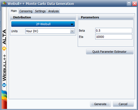
Let us assume that <math>{{t}_{i}}\,\!</math> follows a Weibull distribution with <math>\beta =0.5\,\!</math> and <math>\eta =10000\,\!</math>. The Monte Carlo simulation tool in Weibull++ can be used to generate a set of random numbers that follow a Weibull distribution with the specified parameters. The following picture shows the Main tab of the Monte Carlo Data Generation utility. | |||
[[Image:montecarlo4eva.png|center|450px| ]] | |||
On the Settings tab, set the number of points to '''100''' and click '''Generate'''. This creates a new data sheet in the folio that contains random time values <math>{{t}_{i}}\,\!</math>. | |||
Insert a new data sheet in the folio and enter the corresponding <math>Ln({{t}_{i}})\,\!</math> values of the time values generated by the Monte Carlo simulation. Delete any negative values, if there are any, because Weibull++ expects the time values to be positive. After obtaining the <math>Ln({{t}_{i}})\,\!</math> values, analyze the data sheet using the Gumbel distribution and the MLE parameter estimation method. The estimated parameters are (your results may vary due to the random numbers generated by simulation): | |||
::<math>\begin{align} | ::<math>\begin{align} | ||
& \hat{\mu }= & 9.3816 \\ | & \hat{\mu }= & 9.3816 \\ | ||
& \hat{\sigma }= & 1.9717 | & \hat{\sigma }= & 1.9717 | ||
\end{align}</math> | \end{align}\,\!</math> | ||
Because <math>\ln (\eta )= 9.2103\,\!</math> ( <math>\simeq 9.3816\,\!</math> ) and <math>1/\beta =2\,\!</math> <math>(\simeq 1.9717)\,\!</math>, then this simulation verifies that <math>Ln({{t}_{i}})\,\!</math> follows a Gumbel distribution with <math>\mu =\ln (\eta )\,\!</math> and <math>\delta =1/\beta \,\!</math>. | |||
Note: This example illustrates a property of the Gumbel distribution; it is not meant to be a formal proof. | Note: This example illustrates a property of the Gumbel distribution; it is not meant to be a formal proof. | ||
Revision as of 17:57, 26 September 2012
New format available! This reference is now available in a new format that offers faster page load, improved display for calculations and images and more targeted search.
As of January 2024, this Reliawiki page will not continue to be updated. Please update all links and bookmarks to the latest references at Weibull examples and Weibull reference examples.
This example appears in the Life Data Analysis Reference book.
Verify using Monte Carlo simulation that if [math]\displaystyle{ {{t}_{i}}\,\! }[/math] follows a Weibull distribution with [math]\displaystyle{ \beta \,\! }[/math] and [math]\displaystyle{ \eta \,\! }[/math], then the [math]\displaystyle{ Ln({{t}_{i}})\,\! }[/math] follows a Gumbel distribution with [math]\displaystyle{ \mu =\ln (\eta )\,\! }[/math] and [math]\displaystyle{ \sigma =1/\beta )\,\! }[/math].
Let us assume that [math]\displaystyle{ {{t}_{i}}\,\! }[/math] follows a Weibull distribution with [math]\displaystyle{ \beta =0.5\,\! }[/math] and [math]\displaystyle{ \eta =10000\,\! }[/math]. The Monte Carlo simulation tool in Weibull++ can be used to generate a set of random numbers that follow a Weibull distribution with the specified parameters. The following picture shows the Main tab of the Monte Carlo Data Generation utility.
On the Settings tab, set the number of points to 100 and click Generate. This creates a new data sheet in the folio that contains random time values [math]\displaystyle{ {{t}_{i}}\,\! }[/math].
Insert a new data sheet in the folio and enter the corresponding [math]\displaystyle{ Ln({{t}_{i}})\,\! }[/math] values of the time values generated by the Monte Carlo simulation. Delete any negative values, if there are any, because Weibull++ expects the time values to be positive. After obtaining the [math]\displaystyle{ Ln({{t}_{i}})\,\! }[/math] values, analyze the data sheet using the Gumbel distribution and the MLE parameter estimation method. The estimated parameters are (your results may vary due to the random numbers generated by simulation):
- [math]\displaystyle{ \begin{align} & \hat{\mu }= & 9.3816 \\ & \hat{\sigma }= & 1.9717 \end{align}\,\! }[/math]
Because [math]\displaystyle{ \ln (\eta )= 9.2103\,\! }[/math] ( [math]\displaystyle{ \simeq 9.3816\,\! }[/math] ) and [math]\displaystyle{ 1/\beta =2\,\! }[/math] [math]\displaystyle{ (\simeq 1.9717)\,\! }[/math], then this simulation verifies that [math]\displaystyle{ Ln({{t}_{i}})\,\! }[/math] follows a Gumbel distribution with [math]\displaystyle{ \mu =\ln (\eta )\,\! }[/math] and [math]\displaystyle{ \delta =1/\beta \,\! }[/math].
Note: This example illustrates a property of the Gumbel distribution; it is not meant to be a formal proof.

