Gap Analysis Example

New format available! This reference is now available in a new format that offers faster page load, improved display for calculations and images and more targeted search.

As of January 2024, this Reliawiki page will not continue to be updated. Please update all links and bookmarks to the latest references at RGA examples and RGA reference examples.

---

Consider a system under development that was subjected to a reliability growth test for [math]\displaystyle{ T=1,000\,\! }[/math] hours. Each month, the successive failure times, on a cumulative test time basis, were reported. According to the test plan, 125 hours of test time were accumulated on each prototype system each month. The total reliability growth test program lasted for 7 months. One prototype was tested for each of the months 1, 3, 4, 5, 6 and 7 with 125 hours of test time. During the second month, two prototypes were tested for a total of 250 hours of test time. The next table shows the successive [math]\displaystyle{ N=86\,\! }[/math] failure times that were reported for [math]\displaystyle{ T=1,000\,\! }[/math] hours of testing.

[math]\displaystyle{ {{X}_{i}},\,\! }[/math] [math]\displaystyle{ i=1,2,\ldots ,86\,\! }[/math], [math]\displaystyle{ N = 86, T = 1000\,\! }[/math]

.5	.6	10.7	16.6	18.3	19.2	19.5	25.3
39.2	39.4	43.2	44.8	47.4	65.7	88.1	97.2
104.9	105.1	120.8	195.7	217.1	219	257.5	260.4
281.3	283.7	289.8	306.6	328.6	357.0	371.7	374.7
393.2	403.2	466.5	500.9	501.5	518.4	520.7	522.7
524.6	526.9	527.8	533.6	536.5	542.6	543.2	545.0
547.4	554.0	554.1	554.2	554.8	556.5	570.6	571.4
574.9	576.8	578.8	583.4	584.9	590.6	596.1	599.1
600.1	602.5	613.9	616.0	616.2	617.1	621.4	622.6
624.7	628.8	642.4	684.8	731.9	735.1	753.6	792.5
803.7	805.4	832.5	836.2	873.2	975.1

The observed and cumulative number of failures for each month are:

Month	Time Period	Observed Failure Times	Cumulative Failure Times
1	0-125	19	19
2	125-375	13	32
3	375-500	3	35
4	500-625	38	73
5	625-750	5	78
6	750-875	7	85
7	875-1000	1	86

1. Determine the maximum likelihood estimators for the Crow-AMSAA model.
2. Evaluate the goodness-of-fit for the model.
3. Consider [math]\displaystyle{ (500,\ 625)\,\! }[/math] as the gap interval and determine the maximum likelihood estimates of [math]\displaystyle{ \lambda \,\! }[/math] and [math]\displaystyle{ \beta \,\! }[/math].

Solution

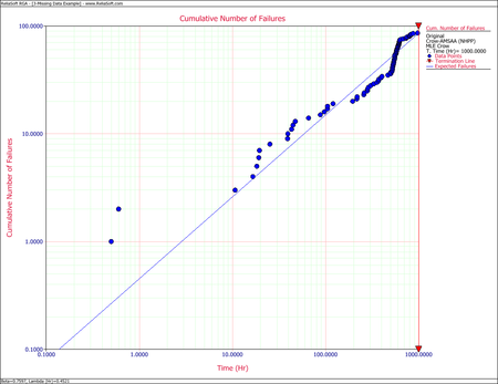
1. For the time terminated test:

   [math]\displaystyle{ \begin{align} & \widehat{\beta }= & 0.7597 \\ & \widehat{\lambda }= & 0.4521 \end{align}\,\! }[/math]

2. The Cramér-von Mises goodness-of-fit test for this data set yields:

   [math]\displaystyle{ C_{M}^{2}=\tfrac{1}{12M}+\underset{i=1}{\overset{M}{\mathop{\sum }}}\,{{\left[ (\tfrac{{{T}_{i}}}{T})\widehat{^{\beta }}-\tfrac{2i-1}{2M} \right]}^{2}}= 0.6989\,\! }[/math]

   The critical value at the 10% significance level is 0.173. Therefore, the test indicated that the analyst should reject the hypothesis that the data set follows the Crow-AMSAA reliability growth model. The following plot shows [math]\displaystyle{ \ln N(t)\,\! }[/math] versus [math]\displaystyle{ \ln t\,\! }[/math] with the fitted line [math]\displaystyle{ \ln \hat{\lambda }+\hat{\beta }\ln t\,\! }[/math], where [math]\displaystyle{ \widehat{\lambda }=0.4521\,\! }[/math] and [math]\displaystyle{ \widehat{\beta }=0.7597\,\! }[/math] are the maximum likelihood estimates.
   

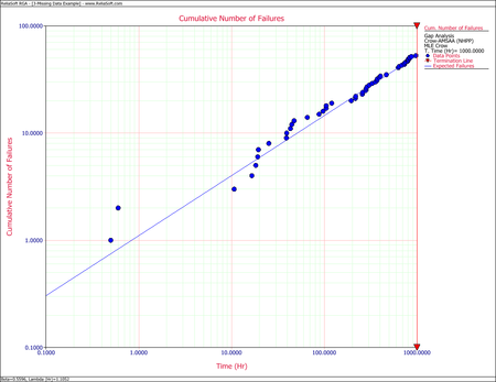
   Observing the data during the fourth month (between 500 and 625 hours), 38 failures were reported. This number is very high in comparison to the failures reported in the other months. A quick investigation found that a number of new data collectors were assigned to the project during this month. It was also discovered that extensive design changes were made during this period, which involved the removal of a large number of parts. It is possible that these removals, which were not failures, were incorrectly reported as failed parts. Based on knowledge of the system and the test program, it was clear that such a large number of actual system failures was extremely unlikely. The consensus was that this anomaly was due to the failure reporting. For this analysis, it was decided that the actual number of failures over this month is assumed to be unknown, but consistent with the remaining data and the Crow-AMSAA reliability growth model.

3. Considering the problem interval [math]\displaystyle{ (500,625)\,\! }[/math] as the gap interval, we will use the data over the interval [math]\displaystyle{ (0,500)\,\! }[/math] and over the interval [math]\displaystyle{ (625,1000).\,\! }[/math] The equations for analyzing missing data are the appropriate equations to estimate [math]\displaystyle{ \lambda \,\! }[/math] and [math]\displaystyle{ \beta \,\! }[/math] because the failure times are known. In this case [math]\displaystyle{ {{S}_{1}}=500,\,{{S}_{2}}=625\,\! }[/math] and [math]\displaystyle{ T=1000,\ {{N}_{1}}=35,\,{{N}_{2}}=13\,\! }[/math]. The maximum likelihood estimates of [math]\displaystyle{ \lambda \,\! }[/math] and [math]\displaystyle{ \beta \,\! }[/math] are:

   [math]\displaystyle{ \begin{align} & \widehat{\beta }= & 0.5596 \\ & \widehat{\lambda }= & 1.1052 \end{align}\,\! }[/math]

   The next figure is a plot of the cumulative number of failures versus time. This plot is approximately linear, which also indicates a good fit of the model.