Accelerated Life Testing and ALTA: Difference between revisions
| Line 170: | Line 170: | ||
::<math></math> | ::<math></math> | ||
<br> | <br> | ||
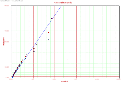
[[Image:cox-snell_plot.gif|thumb|center| | [[Image:cox-snell_plot.gif|thumb|center|400px|Probability plot of the Cox-Snell residuals.]] | ||
<br> | <br> | ||
Revision as of 22:55, 19 August 2011
Accelerated Life Testing and ALTA
This chapter presents issues relevant to using the ALTA software package to analyze data collected in accelerated life tests. These issues include the types of data that can be analyzed and the types of plots that can be created to display analysis results.
Data and Data Types
The analysis of accelerated life tests relies extensively on data. Specifically, analysis relies on life and stress data or times-to-failure data at a specific stress level. The accuracy of any prediction is directly proportional to the quality and accuracy of the supplied data. Good data along with the appropriate distribution and life-stress model usually result in good predictions. Bad or insufficient data will always result in bad predictions.
Most types of non-life data, as well as some life data, are what we term as "complete" data. Complete data means that the value of each sample unit is observed or known. In many cases, however, life data contains uncertainty as to when exactly an event happened (i.e. when the unit failed). Data sets containing such uncertainty as to exactly when the event happened are termed as "censored" data. Each type is explained next.
Complete Data
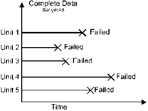
Complete data means that the value of each sample unit is observed (or known) [31]. For example, if we had to compute the average test score for a sample of ten students, complete data would consist of the known score for each student. For life data analysis, known times-to-failure comprise what is usually referred to as complete data. For example, if we tested five units and they all failed, we would then have complete information as to the time-to-failure for each unit in the sample.
Censored Data
There are three types of censored data: right censored, interval censored data and left censored Data. These different types are explained next.
Right Censored (Suspended) Data
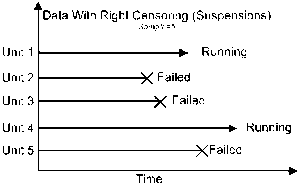
It is also possible that some of the units have not yet failed when the life data are analyzed. This type of data is commonly called right censored data, or suspended data. Assume that we tested five units and three failed. In this scenario, our data set is composed of the times-to-failure of the three units that failed (complete data) and the running time of the other two units that have not failed at the time the data is analyzed (suspended data). This is the most common censoring scheme and it is used extensively in the analysis of field data.
Interval Censored Data
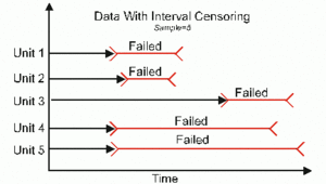
The second type of censoring is commonly called interval censored data. Interval censored data reflects uncertainty as to the exact times the units failed within an interval. This type of data frequently comes from tests or situations where the objects of interest are not constantly monitored. If we are running a test on five units and inspecting them every 100 hours, we only know that a unit failed or did not fail between inspections. More specifically, if we inspect a certain unit at 100 hours and find it is operating and then perform another inspection at 200 hours to find that the unit is no longer operating, we know that a failure occurred in the interval between 100 and 200 hours. In other words, the only information we have is that the unit failed in a certain interval of time. This is also called inspection data by some authors.
Since Interval data is less informative than complete data, it is recomended that they are avoided. This is especially the case in accelerated life tests where a life-stress relationship needs to be determined and interval data affect the accuracy of the fitted relationship, and subsequently the extrapolation to Use conditions. In some cases interval data is unavoidable, due to the nature of the product, the test, and the test equipment, but in these cases caution must be taken to set the inspection intervals to be short enough to observe the spread of the failures. For example, if the inspection interval is too long, all the units in the test may fail within that interval, and thus no failure distribution could be obtained. In accelerated life testing, inspection intervals should be chosen according to the expected acceleration factor at each stress level, and therefore these intervals will be of different length for each stress level.
Left Censored Data
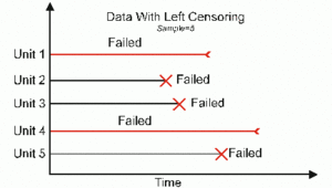
The third type of censoring is similar to the interval censoring and is called left censored data. In left censored data, a failure time is only known to be before a certain time. For instance, we may know that a certain unit failed sometime before 100 hours but not exactly when. In other words, it could have failed any time between 0 and 100 hours. This is identical to interval censored data in which the starting time for the interval is zero.
Grouped Data Analysis
Data can also be entered into ALTA individually or in groups. Grouped data analysis is used for tests in which groups of units possess the same time-to-failure or in which groups of units were suspended at the same time. We highly recommend entering redundant data in groups. Grouped data speeds data entry by the user and significantly speeds up the calculations.
A Note about Complete and Suspended Data
Depending on the event that we want to measure, data type classification (i.e. complete or
suspended) can be open to interpretation. For example, under certain circumstances, and depending
on the question one wishes to answer, a specimen that has failed might be classified as suspended
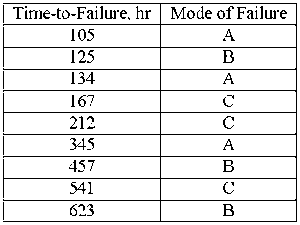
for analysis purposes. To illustrate this, consider the following times-to-failure data for a
product that can fail due to modes A, B and C:
If the objective of analysis is to determine the probability of failure of the product regardless of the mode responsible for the failure, we would analyze the data with all data entries classified as failures (complete data). However, if the objective of the analysis is to determine the probability of failure of the product due to Mode A only, we would then choose to treat failures due to Modes B or C as suspended (right censored) data. Those data points would be treated as suspended data with respect to Mode A because the product operated until the recorded time without failure due to Mode A.
Plots
In addition to the probability plots required in life data analysis, accelerated life test data analysis utilizes a variety of stress-related plots. Each plot provides information crucial to performing accelerated life test analyses. The addition of stress dependency into the life equations introduces another dimension into the plots. This generates a whole new family of 3-dimensional (3D) plots. The following table summarizes the types of plots available in ReliaSoft's ALTA 7 and ALTA 7 PRO .
Considerations relevant to the use of some of the plots available in ALTA are discussed in the sections that follow.
Probability Plots
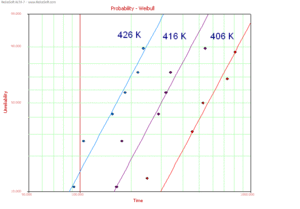
The probability plots used in accelerated life testing data analysis are similar to those used in life data analysis. The only difference is that each probability plot in accelerated testing is associated with the corresponding stress or stresses. Multiple lines will be plotted on a probability plot in ALTA, each corresponding to a different stress level. The information that can be obtained from probability plots includes: reliability with confidence bounds, warranty time with confidence bounds, shape and scale parameters, etc.
Reliability and Unreliability Plots
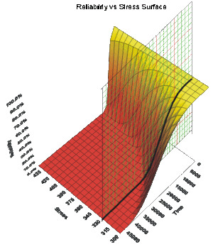
There are two types of reliability plots. The first type is a 2-dimensional plot of Reliability vs. Time for a given stress level. The second type is a 3-dimensional plot of the Reliability vs. Time vs. Stress. The 2-dimensional plot of reliability is just a section of the 3-dimensional plot at the desired stress level, as illustrated in Figure 2.
A Reliability vs. Time plot provides reliability values at a given time and time at a given reliability. These can be plotted with or without confidence bounds. The same 2-dimensional and 3-dimensional plots are available for unreliability as well, and they are just the complement of the reliability plots.
Failure Rate Plots
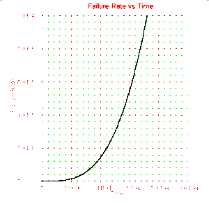
The instantaneous failure rate is a function of time and stress. For this reason, a 2-dimensional plot of Failure Rate vs. Time at a given stress and a 3-dimensional plot of Failure Rate vs. Time and Stress can be obtained in ALTA.
A failure rate plot shows the expected number of failures per unit time at a particular stress level (e.g. failures per hour at 410K).
Pdf Plots
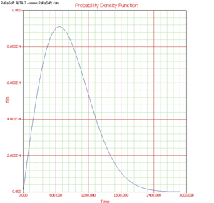
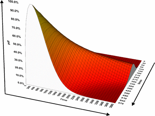
The [math]\displaystyle{ pdf }[/math] is a function of time and stress. For this reason, a 2-dimensional plot of the [math]\displaystyle{ pdf }[/math] vs. Time at a given stress and a 3-dimensional plot of the [math]\displaystyle{ pdf }[/math] vs. Time and Stress can be obtained in ALTA.
A [math]\displaystyle{ pdf }[/math] plot represents the relative frequency of failures as a function of time and stress. Although the [math]\displaystyle{ pdf }[/math] plot is less important in most reliability applications than the other plots available in ALTA, it provides a good way of visualizing the distribution and its characteristics such as its shape, skewness, mode, etc.
Life-Stress Plots
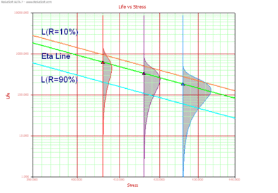
Life vs. Stress plots and Probability plots are the most important plot types in accelerated life testing analysis. Life vs. Stress plots are widely used for estimating the parameters of life-stress relationships. Any life measure can be plotted versus stress in the Life vs. Stress plots available in ALTA. Confidence bounds information on each life measure can also be plotted. The most widely used Life vs. Stress plots are the Arrhenius and the inverse power law plots. Fig. 7 illustrates a typical Arrhenius Life vs. Stress plot.
Each line in Fig. 7 represents the path for extrapolating a life measure, such as a percentile, from one stress level to another. The slope and intercept of those lines are the parameters of the life-stress relationship (whenever the relationship can be linearized). The imposed pdfs represent the distribution of the data at each stress level.
Standard Deviation Plots
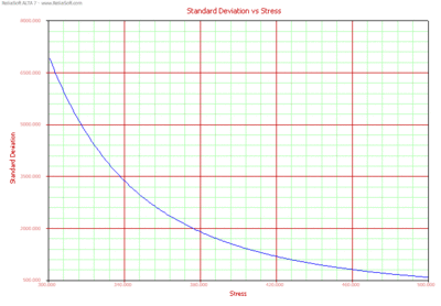
Standard Deviation vs. Stress is a useful plot in accelerated life testing analysis and provides information about the spread of the data at each stress level.
Acceleration Factor Plots
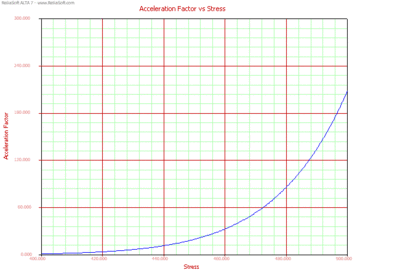
The acceleration factor is a unitless number that relates a product's life at an accelerated stress level to the life at the use stress level. It is defined by:
- [math]\displaystyle{ {{A}_{F}}=\frac{{{L}_{u}}}{{{L}_{A}}} }[/math]
- where:
- • [math]\displaystyle{ {{L}_{u}} }[/math] is the life at the use stress level.
- • [math]\displaystyle{ {{L}_{A}} }[/math] is the life at the accelerated level.
As it can be seen in Eqn. (af), the acceleration factor depends on the life-stress relationship (i.e. Arrhenius, Eyring, etc.), and is thus a function of stress.
The Acceleration Factor vs. Stress plot is generated using Eqn. (af) at a constant use stress level and at a varying accelerated stress. In Figure 9, the Acceleration Factor vs. Stress was plotted for a constant use level of 300K. Since [math]\displaystyle{ {{L}_{A}}={{L}_{u}} }[/math] , the value of the acceleration factor at 300K is equal to 1. The acceleration factor for a temperature of 450K is approximately 8. This means that the life at the use level of 300K is eight times higher than the life at 450K.
Residual Plots
Residual analysis for reliability consists of analyzing the results of a regression analysis by assigning residual values to each data point in the data set. Plotting these residuals provides a very good tool in assessing model assumptions and revealing inadequacies in the model, as well as revealing extreme observations. Three types of residual plots are available in ALTA.
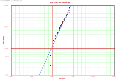
Standardized Residuals (SR)
The standardized residuals plot for the Weibull and lognormal distributions can be obtained in ALTA. Each plot type is discussed next.
SR for the Weibull Distribution
Once the parameters have been estimated, the standardized residuals for the Weibull distribution can be calculated by:
- [math]\displaystyle{ {{\widehat{e}}_{i}}=\widehat{\beta }\left[ \ln ({{T}_{i}})-\ln (\widehat{\eta }(V)) \right] }[/math]
Then, under the assumed model, these residuals should look like a sample from an extreme value distribution with a mean of 0. For the Weibull distribution the standardized residuals are plotted on a smallest extreme value probability paper. If the Weibull distribution adequately describes the data, then the standardized residuals should appear to follow a straight line on such a probability plot. Note that when an observation is censored (suspended), the corresponding residual is also censored.
SR for the Lognormal Distribution
Once the parameters have been estimated using rank regression, the fitted or calculated responses can be calculated by:
- [math]\displaystyle{ {{\widehat{e}}_{i}}=\frac{\ln ({{T}_{i}})-{{\widehat{\mu }}^{\prime }}}{{{\widehat{\sigma }}_{{{T}'}}}} }[/math]
Then, under the assumed model, the standardized residuals should be normally distributed with a mean of 0 and a standard deviation of 1 ( [math]\displaystyle{ \tilde{\ }N(0,1) }[/math] ). Consequently, the standardized residuals for the lognormal distribution are commonly displayed on a normal probability plot.
Cox-Snell Residuals
The Cox-Snell residuals are given by:
- [math]\displaystyle{ {{\widehat{e}}_{i}}=-\ln [R({{T}_{i}})] }[/math]
where [math]\displaystyle{ R({{T}_{i}}) }[/math] is the calculated reliability value at failure time [math]\displaystyle{ {{T}_{i}}. }[/math] The Cox-Snell residuals are plotted on an exponential probability paper.
- [math]\displaystyle{ }[/math]
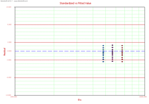
Standardized vs Fitted Values
A Standardized vs. Fitted Value plot helps to detect behavior not modeled in the underlying relationship. However, when heavy censoring is present, the plot is more difficult to interpret. In a Standardized vs. Fitted Value plot, the standardized residuals are plotted versus the scale parameter of the underlying life distribution (which is a function of stress) on log-linear paper (linear on the Y-axis). Therefore, in the case of the Weibull distribution, the standardized residuals are plotted versus [math]\displaystyle{ \eta (V), }[/math] for the lognormal versus [math]\displaystyle{ {\mu }'(V), }[/math] and for the exponential versus [math]\displaystyle{ m(V). }[/math]
| The material on this page is copyrighted. | ©1992-2012. ReliaSoft Corporation. ALL RIGHTS RESERVED. |

