Template:Weibull parameters rank regression on x

Rank Regression on X

Performing a rank regression on X is similar to the process for rank regression on Y, with the difference being that the horizontal deviations from the points to the line are minimized rather than the vertical. Again, the first task is to bring our function, Eqn. (EQNREF Fw ), into a linear form. This step is exactly the same as in the regression on Y analysis and Eqns. (EQNREF logw ), (EQNREF yw ), (EQNREF aw ) and (EQNREF bw ) apply in this case too. The derivation from the previous analysis begins on the least squares fit part, where in this case we treat as the dependent variable and as the independent variable. The best-fitting straight line to the data, for regression on X (see Chapter 3), is the straight line:

[math]\displaystyle{ x= \hat{a}+\hat{b}y }[/math] EQNREF xlinew

The corresponding equations for [math]\displaystyle{ \hat{a} }[/math] and [math]\displaystyle{ \hat{b} }[/math] are:

[math]\displaystyle{ \hat{a}=\overline{x}-\hat{b}\overline{y}=\frac{\sum\limits_{i=1}^{N}x_{i}}{N} -\hat{b}\frac{\sum\limits_{i=1}^{N}y_{i}}{N} }[/math]

and

[math]\displaystyle{ \hat{b}={\frac{\sum\limits_{i=1}^{N}x_{i}y_{i}-\frac{\sum \limits_{i=1}^{N}x_{i}\sum\limits_{i=1}^{N}y_{i}}{N}}{\sum \limits_{i=1}^{N}y_{i}^{2}-\frac{\left( \sum\limits_{i=1}^{N}y_{i}\right) ^{2}}{N}}} }[/math]

where:

[math]\displaystyle{ y_{i}=\ln \left\{ -\ln [1-F(T_{i})]\right\} }[/math] and:

x_i = ln(T_i) and the F(T_i) values are again obtained from the median ranks.

Once [math]\displaystyle{ \hat{a} }[/math] and [math]\displaystyle{ \hat{b} }[/math] are obtained, solve Eqn. (EQNREF xlinew ) for y, which corresponds to:

[math]\displaystyle{ y=-\frac{\hat{a}}{\hat{b}}+\frac{1}{\hat{b}}x }[/math] Solving for the parameters from Eqns. (EQNREF aw ) and (EQNREF bw ) we get

[math]\displaystyle{ a=-\frac{\hat{a}}{\hat{b}}=-\beta \ln (\eta ) }[/math] EQNREF awx

and

[math]\displaystyle{ b=\frac{1}{\hat{b}}=\beta EQNREF bwx }[/math] The correlation coefficient is evaluated as before using Eqn. (EQNREF RHOw ).

Example 4: 2P Weibull Distribution RRX Example

Repeat Example 1 using rank regression on X.

Solution

Solution to Example 4 Table 8.1, constructed in Example 3, can also be applied to this example.

Using the values from this table we get:

[math]\displaystyle{ \hat{b} ={\frac{\sum\limits_{i=1}^{6}(\ln T_{i})y_{i}-\frac{ \sum\limits_{i=1}^{6}\ln T_{i}\sum\limits_{i=1}^{6}y_{i}}{6}}{ \sum\limits_{i=1}^{6}y_{i}^{2}-\frac{\left( \sum\limits_{i=1}^{6}y_{i}\right) ^{2}}{6}}} }[/math]

[math]\displaystyle{ \hat{b} =\frac{-8.0699-(23.9068)(-3.0070)/6}{7.1502-(-3.0070)^{2}/6} }[/math]

or:

[math]\displaystyle{ \hat{b}=0.6931 }[/math]

and:

[math]\displaystyle{ \hat{a}=\overline{x}-\hat{b}\overline{y}=\frac{\sum\limits_{i=1}^{6}\ln T_{i} }{6}-\hat{b}\frac{\sum\limits_{i=1}^{6}y_{i}}{6} }[/math]

or:

[math]\displaystyle{ \hat{a}=\frac{23.9068}{6}-(0.6931)\frac{(-3.0070)}{6}=4.3318 }[/math]

Therefore, from Eqn. (EQNREF bwx ):

[math]\displaystyle{ \hat{\beta }=\frac{1}{\hat{b}}=\frac{1}{0.6931}=1.4428 }[/math]

and from Eqn. (EQNREF awx )

[math]\displaystyle{ \hat{\eta }=e^{\frac{\hat{a}}{\hat{b}}\cdot \frac{1}{\hat{ \beta }}}=e^{\frac{4.3318}{0.6931}\cdot \frac{1}{1.4428}}=76.0811\text{ hr} }[/math]

The correlation coefficient is found using Eqn. (EQNREF RHOw ):

[math]\displaystyle{ \hat{\rho }=0.9956 }[/math]

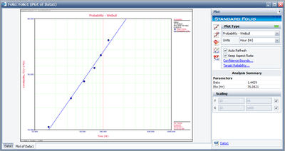
The results and the associated graph using Weibull++ are given next. Note that the slight variation in the results is due to the number of significant figures used in the estimation of the median ranks. Weibull++ by default uses double precision accuracy when computing the median ranks.