Template:Crow discrete reliability growth model camsaa
Crow Discrete Reliability Growth Model
The Crow-AMSAA model can be adapted for the analysis of success/failure data (also called "discrete" or "attribute" data).
Model Development
Suppose system development is represented by [math]\displaystyle{ i }[/math] configurations. This corresponds to [math]\displaystyle{ i-1 }[/math] configuration changes, unless fixes are applied at the end of the test phase, in which case there would be [math]\displaystyle{ i }[/math] configuration changes. Let [math]\displaystyle{ {{N}_{i}} }[/math] be the number of trials during configuration [math]\displaystyle{ i }[/math] and let [math]\displaystyle{ {{M}_{i}} }[/math] be the number of failures during configuration [math]\displaystyle{ i }[/math] . Then the cumulative number of trials through configuration [math]\displaystyle{ i }[/math] , namely [math]\displaystyle{ {{T}_{i}} }[/math] , is the sum of the [math]\displaystyle{ {{N}_{i}} }[/math] for all [math]\displaystyle{ i }[/math] , or:
- [math]\displaystyle{ {{T}_{i}}=\underset{}{\overset{}{\mathop \sum }}\,{{N}_{i}} }[/math]
And the cumulative number of failures through configuration [math]\displaystyle{ i }[/math] , namely [math]\displaystyle{ {{K}_{i}} }[/math] , is the sum of the [math]\displaystyle{ {{M}_{i}} }[/math] for all [math]\displaystyle{ i }[/math] , or:
- [math]\displaystyle{ {{K}_{i}}=\underset{}{\overset{}{\mathop \sum }}\,{{M}_{i}} }[/math]
The expected value of [math]\displaystyle{ {{K}_{i}} }[/math] can be expressed as [math]\displaystyle{ E[{{K}_{i}}] }[/math] and defined as the expected number of failures by the end of configuration [math]\displaystyle{ i }[/math] . Applying the learning curve property to [math]\displaystyle{ E[{{K}_{i}}] }[/math] implies:
- [math]\displaystyle{ E\left[ {{K}_{i}} \right]=\lambda T_{i}^{\beta } }[/math]
Denote [math]\displaystyle{ {{f}_{1}} }[/math] as the probability of failure for configuration 1 and use it to develop a generalized equation for [math]\displaystyle{ {{f}_{i}} }[/math] in terms of the [math]\displaystyle{ {{T}_{i}} }[/math] and [math]\displaystyle{ {{N}_{i}} }[/math] . From Eqn. (expectedn), the expected number of failures by the end of configuration 1 is:
- [math]\displaystyle{ E\left[ {{K}_{1}} \right]=\lambda T_{1}^{\beta }={{f}_{1}}{{N}_{1}} }[/math]
- [math]\displaystyle{ \therefore {{f}_{1}}=\frac{\lambda T_{1}^{\beta }}{{{N}_{1}}} }[/math]
Applying Eqn. (expectedn) again and noting that the expected number of failures by the end of configuration 2 is the sum of the expected number of failures in configuration 1 and the expected number of failures in configuration 2:
- [math]\displaystyle{ \begin{align} & E\left[ {{K}_{2}} \right]= & \lambda T_{2}^{\beta } \\ & = & {{f}_{1}}{{N}_{1}}+{{f}_{2}}{{N}_{2}} \\ & = & \lambda T_{1}^{\beta }+{{f}_{2}}{{N}_{2}} \end{align} }[/math]
- [math]\displaystyle{ \therefore {{f}_{2}}=\frac{\lambda T_{2}^{\beta }-\lambda T_{1}^{\beta }}{{{N}_{2}}} }[/math]
By this method of inductive reasoning, a generalized equation for the failure probability on a configuration basis, [math]\displaystyle{ {{f}_{i}} }[/math] , is obtained, such that:
- [math]\displaystyle{ {{f}_{i}}=\frac{\lambda T_{i}^{\beta }-\lambda T_{i-1}^{\beta }}{{{N}_{i}}} }[/math]
For the special case where [math]\displaystyle{ {{N}_{i}}=1 }[/math] for all [math]\displaystyle{ i }[/math] , Eqn. (dfi) becomes a smooth curve, [math]\displaystyle{ {{g}_{i}} }[/math] , that represents the probability of failure for trial by trial data, or:
- [math]\displaystyle{ {{g}_{i}}=\lambda \cdot {{i}^{\beta }}-\lambda \cdot {{\left( i-1 \right)}^{\beta }} }[/math]
In Eqn. (dfi1), [math]\displaystyle{ i }[/math] represents the trial number. Thus using Eqn. (dfi), an equation for the reliability (probability of success) for the [math]\displaystyle{ {{i}^{th}} }[/math] configuration is obtained:
- [math]\displaystyle{ {{R}_{i}}=1-{{f}_{i}} }[/math]
And using Eqn. (dfi1), the equation for the reliability for the [math]\displaystyle{ {{i}^{th}} }[/math] trial is:
- [math]\displaystyle{ {{R}_{i}}=1-{{g}_{i}} }[/math]
Maximum Likelihood Estimators
This section describes procedures for estimating the parameters of the Crow-AMSAA model for success/failure data. An example is presented illustrating these concepts. The estimation procedures described below provide maximum likelihood estimates (MLEs) for the model's two parameters, [math]\displaystyle{ \lambda }[/math] and [math]\displaystyle{ \beta }[/math] . The MLEs for [math]\displaystyle{ \lambda }[/math] and [math]\displaystyle{ \beta }[/math] allow for point estimates for the probability of failure, given by:
- [math]\displaystyle{ {{\hat{f}}_{i}}=\frac{\hat{\lambda }T_{i}^{{\hat{\beta }}}-\hat{\lambda }T_{i-1}^{{\hat{\beta }}}}{{{N}_{i}}}=\frac{\hat{\lambda }\left( T_{i}^{{\hat{\beta }}}-T_{i-1}^{{\hat{\beta }}} \right)}{{{N}_{i}}} }[/math]
And the probability of success (reliability) for each configuration [math]\displaystyle{ i }[/math] is equal to:
- [math]\displaystyle{ {{\hat{R}}_{i}}=1-{{\hat{f}}_{i}} }[/math]
The likelihood function is:
- [math]\displaystyle{ \underset{i=1}{\overset{k}{\mathop \prod }}\,\left( \begin{matrix} {{N}_{i}} \\ {{M}_{i}} \\ \end{matrix} \right){{\left( \frac{\lambda T_{i}^{\beta }-\lambda T_{i-1}^{\beta }}{{{N}_{i}}} \right)}^{{{M}_{i}}}}{{\left( \frac{{{N}_{i}}-\lambda T_{i}^{\beta }+\lambda T_{i-1}^{\beta }}{{{N}_{i}}} \right)}^{{{N}_{i}}-{{M}_{i}}}} }[/math]
Taking the natural log on both sides yields:
- [math]\displaystyle{ \begin{align} & \Lambda = & \underset{i=1}{\overset{K}{\mathop \sum }}\,\left[ \ln \left( \begin{matrix} {{N}_{i}} \\ {{M}_{i}} \\ \end{matrix} \right)+{{M}_{i}}\left[ \ln (\lambda T_{i}^{\beta }-\lambda T_{i-1}^{\beta })-\ln {{N}_{i}} \right] \right] \\ & & +\underset{i=1}{\overset{K}{\mathop \sum }}\,\left[ ({{N}_{i}}-{{M}_{i}})\left[ \ln ({{N}_{i}}-\lambda T_{i}^{\beta }+\lambda T_{i-1}^{\beta })-\ln {{N}_{i}} \right] \right] \end{align} }[/math]
Taking the derivative with respect to [math]\displaystyle{ \lambda }[/math] and [math]\displaystyle{ \beta }[/math] respectively, exact MLEs for [math]\displaystyle{ \lambda }[/math] and [math]\displaystyle{ \beta }[/math] are values satisfying the following two equations:
- [math]\displaystyle{ \begin{align} & \underset{i=1}{\overset{K}{\mathop \sum }}\,{{H}_{i}}\times {{S}_{i}}= & 0 \\ & \underset{i=1}{\overset{K}{\mathop \sum }}\,{{U}_{i}}\times {{S}_{i}}= & 0 \end{align} }[/math]
- where:
- [math]\displaystyle{ \begin{align} & {{H}_{i}}= & \underset{i=1}{\overset{K}{\mathop \sum }}\,\left[ T_{i}^{\beta }\ln {{T}_{i}}-T_{i-1}^{\beta }\ln {{T}_{i-1}} \right] \\ & {{S}_{i}}= & \frac{{{M}_{i}}}{\left[ \lambda T_{i}^{\beta }-\lambda T_{i-1}^{\beta } \right]}-\frac{{{N}_{i}}-{{M}_{i}}}{\left[ {{N}_{i}}-\lambda T_{i}^{\beta }+\lambda T_{i-1}^{\beta } \right]} \\ & {{U}_{i}}= & T_{i}^{\beta }-T_{i-1}^{\beta }\, \end{align} }[/math]
Example 8
A one-shot system underwent reliability growth development testing for a total of 68 trials. Delayed corrective actions were incorporated after the 14th, 33rd and 48th trials. From trial 49 to trial 68, the configuration was not changed.
• Configuration 1 experienced 5 failures,
• Configuration 2 experienced 3 failures,
• Configuration 3 experienced 4 failures and
• Configuration 4 experienced 4 failures.
- 1) Estimate the parameters of the Crow-AMSAA model using maximum likelihood estimation.
- 2) Estimate the unreliability and reliability by configuration.
Solution
- 1) The solution of Eqns. (solution1) and (solution2) provides for [math]\displaystyle{ \lambda }[/math] and [math]\displaystyle{ \beta }[/math] corresponding to 0.5954 and 0.7801, respectively.
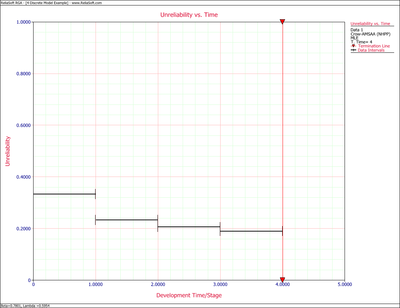
- 2) Table 5.6 displays the results of Eqns. (ffffi) and (rrrri).
Figures 4fig816 and 4fig817 show plots of the estimated unreliability and reliability by configuration.
| Configuration([math]\displaystyle{ i }[/math]) | Estimated Failure Probability | Estimated Reliability |
|---|---|---|
| 1 | 0.333 | 0.667 |
| 2 | 0.234 | 0.766 |
| 3 | 0.206 | 0.794 |
| 4 | 0.190 | 0.810 |
Mixed Data
In the RGA Software, the Discrete Data > Mixed Data option gives a data sheet that can have input data that is either configuration in groups or individual trial by trial, or a mixed combination of individual trials and configurations of more than one trial. The calculations use the same mathematical methods described in section 5.3 for the Crow-AMSAA grouped data.
Example 9
Table 5.7 shows the number of fai
[math]\displaystyle{ \widehat{\beta }=0.7950 }[/math]
lures of each interval of trials and the cumulative number of trials in each interval for a reliability growth test. For example, the first row of Table 5.7 indicates that for an interval of 14 trials, 5 failures occurred.
| Failures in Interval | Cumulative Trials |
|---|---|
| 5 | 14 |
| 3 | 33 |
| 4 | 48 |
| 0 | 52 |
| 1 | 53 |
| 0 | 57 |
| 1 | 58 |
| 0 | 62 |
| 1 | 63 |
| 0 | 67 |
| 1 | 68 |
Using RGA 7, the parameters of the Crow-AMSAA model are estimated as follows:
- and:
- [math]\displaystyle{ \widehat{\lambda }=0.5588 }[/math]
As we have seen, the Crow-AMSAA instantaneous failure intensity, [math]\displaystyle{ {{\lambda }_{i}}(T) }[/math] , is defined as:
- [math]\displaystyle{ {{\lambda }_{i}}(T)=\lambda \beta {{T}^{\beta -1}},\text{with }T\gt 0,\text{ }\lambda \gt 0\text{ and }\beta \gt 0 }[/math]
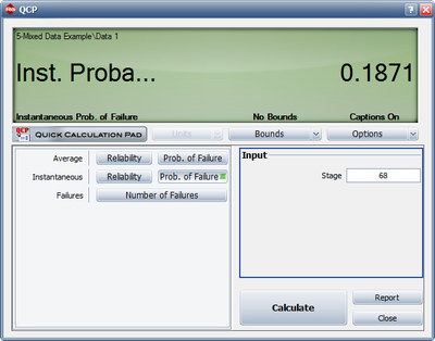
Using the above parameter estimates, we can calculate the or instantaneous unreliability at the end of the test, or [math]\displaystyle{ T=68. }[/math]
- [math]\displaystyle{ {{R}_{i}}(68)=0.5588\cdot 0.7950\cdot {{68}^{0.7950-1}}=0.1871 }[/math]
This result that can be obtained from the Quick Calculation Pad (QCP), for [math]\displaystyle{ T=68, }[/math] as seen in Figure Mixednst.FI.
The instantaneous reliability can then be calculated as:
- [math]\displaystyle{ {{R}_{inst}}=1-0.1871=0.8129 }[/math]
The average unreliability is calculated as:
- [math]\displaystyle{ \text{Average Unreliability }({{t}_{1,}}{{t}_{2}})=\frac{\lambda t_{2}^{\beta }-\lambda t_{1}^{\beta }}{{{t}_{2}}-{{t}_{1}}} }[/math]
and the average reliability is calculated as:
- [math]\displaystyle{ \text{Average Reliability }({{t}_{1,}}{{t}_{2}})=1-\frac{\lambda t_{2}^{\beta }-\lambda t_{1}^{\beta }}{{{t}_{2}}-{{t}_{1}}} }[/math]
Bounds on Average Failure Probability for Mixed Data
The process to calculate the average unreliability confidence bounds for mixed data is as follows:
- 1) Calculate the average failure probability .
- 2) There will exist a [math]\displaystyle{ {{t}^{*}} }[/math] between [math]\displaystyle{ {{t}_{1}} }[/math] and [math]\displaystyle{ {{t}_{2}} }[/math] such that the instantaneous unreliability at [math]\displaystyle{ {{t}^{*}} }[/math] equals the average unreliability . The confidence intervals for the instantaneous unreliability at [math]\displaystyle{ {{t}^{*}} }[/math] are the confidence intervals for the average unreliability .
Bounds on Average Reliability for Mixed Data
The process to calculate the average reliability confidence bounds for mixed data is as follows:
- 1) Calculate confidence bounds for average unreliability as described above.
- 2) The confidence bounds for reliability are 1 minus these confidence bounds for average unreliability.


