Template:Normal distribution probability plotting

Probability Plotting

As described before, probability plotting involves plotting the failure times and associated unreliability estimates on specially constructed probability plotting paper. The form of this paper is based on a linearization of the [math]\displaystyle{ cdf }[/math] of the specific distribution. For the normal distribution, the cumulative density function can be written as:

[math]\displaystyle{ F(T)=\Phi \left( \frac{T-\mu }{{{\sigma }_{T}}} \right) }[/math]

or:

[math]\displaystyle{ {{\Phi }^{-1}}\left[ F(T) \right]=-\frac{\mu}{\sigma}+\frac{1}{\sigma}T }[/math]

where:

[math]\displaystyle{ \Phi (x)=\frac{1}{\sqrt{2\pi }}\int_{-\infty }^{x}{{e}^{-\tfrac{{{t}^{2}}}{2}}}dt }[/math]

Now, let:

[math]\displaystyle{ y={{\Phi }^{-1}}\left[ F(T) \right] }[/math]

[math]\displaystyle{ a=-\frac{\mu }{\sigma } }[/math]

and:

[math]\displaystyle{ b=\frac{1}{\sigma } }[/math]

which results in the linear equation of:

[math]\displaystyle{ y=a+bT }[/math]

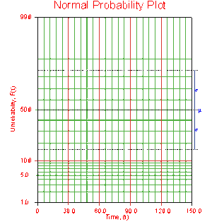
The normal probability paper resulting from this linearized [math]\displaystyle{ cdf }[/math] function is shown next.

Since the normal distribution is symmetrical, the area under the [math]\displaystyle{ pdf }[/math] curve from [math]\displaystyle{ -\infty }[/math] to [math]\displaystyle{ \mu }[/math] is [math]\displaystyle{ 0.5 }[/math] , as is the area from [math]\displaystyle{ \mu }[/math] to [math]\displaystyle{ +\infty }[/math] . Consequently, the value of [math]\displaystyle{ \mu }[/math] is said to be the point where [math]\displaystyle{ R(t)=Q(t)=50% }[/math] . This means that the estimate of [math]\displaystyle{ \mu }[/math] can be read from the point where the plotted line crosses the 50% unreliability line.

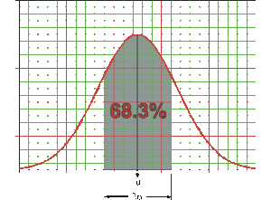
To determine the value of [math]\displaystyle{ \sigma }[/math] from the probability plot, it is first necessary to understand that the area under the [math]\displaystyle{ pdf }[/math] curve that lies between one standard deviation in either direction from the mean (or two standard deviations total) represents 68.3% of the area under the curve. This is represented graphically in the following figure.

Consequently, the interval between [math]\displaystyle{ Q(t)=84.15% }[/math] and [math]\displaystyle{ Q(t)=15.85% }[/math] represents two standard deviations, since this is an interval of 68.3% ( [math]\displaystyle{ 84.15-15.85=68.3 }[/math] ), and is centered on the mean at 50%. As a result, the standard deviation can be estimated from:

[math]\displaystyle{ \widehat{\sigma }=\frac{t(Q=84.15%)-t(Q=15.85%)}{2} }[/math]

That is: the value of [math]\displaystyle{ \widehat{\sigma } }[/math] is obtained by subtracting the time value where the plotted line crosses the 84.15% unreliability line from the time value where the plotted line crosses the 15.85% unreliability line and dividing the result by two. This process is illustrated in the following example.