Basic Statistical Background

Statistical Background

In this section provides a brief elementary introduction to the most common and fundamental statistical equations and definitions used in reliability engineering and life data analysis.

Random Variables

In general, most problems in reliability engineering deal with quantitative measures, such as the time-to-failure of a component, or whether the component fails or does not fail. In judging a component to be defective or non-defective, only two outcomes are possible. We can then denote a random variable X as representative of these possible outcomes (i.e. defective or non-defective). In this case, X is a random variable that can only take on these values.

In the case of times-to-failure, our random variable X can take on the time-to-failure (or time to an event of interest) of the product or component and can be in a range from 0 to infinity (since we do not know the exact time a priori).

In the first case, where the random variable can take on only two discrete values (let's say defective =0 and non-defective=1>), the variable is said to be a discrete random variable. In the second case, our product can be found failed at any time after time 0, i.e. at 12.4 hours or at 100.12 miles and so forth, thus X can take on any value in this range. In this case, our random variable X is said to be a continuous random variable.

The Probability Density and Cumulative Distribution Functions

Designations

From probability and statistics, given a continuous random variable, we denote:

• The probability density function, pdf, as f(x).

• The cumulative distribution function, cdf, as F(x).

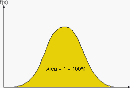
The pdf and cdf give a complete description of the probability distribution of a random variable.

Definitions

If $X$ is a continuous random variable, then the probability density function, $pdf$, of $X$, is a function $f(x)$ such that for two numbers, $a$ and $b$ with $a\le b$:

$P(a\le X\le b)={\int }_a^{b}f(x)dx$ and $f(x)\ge 0$ for all x

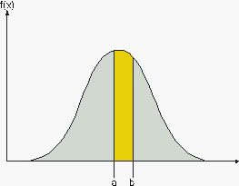
That is, the probability that takes on a value in the interval [a,b] is the area under the density function from $a$ to $b$. The cumulative distribution function, $cdf$, is a function $F(x)$ of a random variable, $X$, and is defined for a number $x$ by:

$F(x)=P(X\le x)={\int }_0^{\mathrm{\infty }}xf(s)ds$

That is, for a given value $x$, $F(x)$ is the probability that the observed value of $X$ will be at most $x$. Note that the limits of integration depend on the domain of $f(x)$. For example, for all the distributions considered in this reference, this domain would be $[0,+\mathrm{\infty }]$, $[-\mathrm{\infty },+\mathrm{\infty }]$ or $[\gamma ,+\mathrm{\infty }]$. In the case of $[\gamma ,+\mathrm{\infty }]$, we use the constant $\gamma$ to denote an arbitrary non-zero point (or a location that indicates the starting point for the distribution). Figure 3-1, on the next page, illustrates the relationship between the probability density function and the cumulative distribution function.

Figure 3.1: A graphical representation of the relationship between the pdf and cdf.

Mathematical Relationship Between the $pdf$ and $cdf$

The mathematical relationship between the $pdf$ and $cdf$ is given by:

$F(x)={\int }_{-\mathrm{\infty }}^{x}f(s)ds$

Conversely:

$f(x)=\frac{d(F(x))}{dx}$

In plain English, the value of the $cdf$ at $x$ is the area under the probability density function up to $x$, if so chosen. It should also be pointed out that the total area under the $pdf$ is always equal to 1, or mathematically:

${\int }_{-\mathrm{\infty }}^{\mathrm{\infty }}f(x)dx=1$

An example of a probability density function is the well-known normal distribution, whose $pdf$ is given by:

$f(t)=\frac{1}{\sigma \sqrt{2\pi }}{e}^{-\frac{1}{2}}(\frac{t-\mu }{\sigma }{)}^2$

where $\mu$ is the mean and .. is the standard deviation. The normal distribution is a two-parameter distribution, i.e. with two parameters $\mu$ and $\sigma$. Another two-parameter distribution is the lognormal distribution, whose $pdf$ is given by:

$f(t)=\frac{1}{t\cdot {\sigma }^{\prime }\sqrt{2\pi }}{e}^{-\frac{1}{2}(\frac{t^{\prime }-{\mu }^{\prime }}{{\sigma }^{\prime }}{)}^2}$

where $t^{\prime }$ is the natural logarithm of the times-to-failure, ${\mu }^{\prime }$ is the mean of the natural logarithms of the times-to-failure and ${\sigma }^{\prime }$ is the standard deviation of the natural logarithms of the times-to-failure, $t^{\prime }$.

The Reliability Function

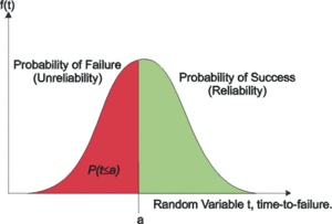
The reliability function can be derived using the previous definition of the cumulative distribution function, Eqn. (e21). The probability of an event happening by time $t$ is given by:

$F(t)={\int }_{0,\gamma }^{t}f(s)ds$

In particular, this represents the probability of a unit failing by time $t$. From this, we obtain the most commonly used function in reliability engineering, the reliability function, which represents the probability of success of a unit in undertaking a mission of a prescribed duration. To mathematically show this, we first define the unreliability function, $Q(t)$, which is the probability of failure, or the probability that our time-to-failure is in the region of $0$ (or $\gamma$) and $t$. So from Eqn.(ee34):

$F(t)=Q(t)={\int }_{0,\gamma }^{t}f(s)ds$

In this situation, there are only two states that can occur: success or failure. These two states are also mutually exclusive. Since reliability and unreliability are the probabilities of these two mutually exclusive states, the sum of these probabilities is always equal to unity. So then:

$\begin{array}{rl}Q(t)+R(t)& =1\\ R(t)& =1-Q(t)\\ R(t)& =1-{\int }_{0,\gamma }^{t}f(s)ds\\ R(t)& ={\int }_t^{\mathrm{\infty }}f(s)ds\end{array}$

Conversely:

$f(t)=-\frac{d(R(t))}{dt}$

The Conditional Reliability Function

The reliability function discussed previously assumes that the unit is starting the mission with no accumulated time, i.e. brand new. Conditional reliability calculations allow one to calculate the probability of a unit successfully completing a mission of a particular duration given that it has already successfully completed a mission of a certain duration. In this respect, the conditional reliability function could be considered to be the reliability of used equipmen.

The conditional reliability function is given by the equation,

$R(t|T)=\frac{R(T+t)}{R(T)}$

where:

• t is the duration of the new mission, and
• T is the duration of the successfully completed previous mission.

In other words, the fact that the equipment has already successfully completed a mission, $T$, tells us that the product successfully traversed the failure rate path for the period from $0\to T$, and it will now be failing according to the failure rate from $T\to T+t$ . This is used when analyzing warranty data (Chapter 11).

The Failure Rate Function

The failure rate function enables the determination of the number of failures occurring per unit time. Omitting the derivation (see [19; Chapter 4]), the failure rate is mathematically given as,

$\begin{array}{rl}\lambda (t)& =\frac{f(t)}{1-{\int }_{0,\gamma }^{t}f(s)ds}\\ & =\frac{f(t)}{R(t)}\end{array}$

The failure rate function has the units of failures per unit time among surviving, e.g. 1 failure per month.

The Mean Life Function

The mean life function, which provides a measure of the average time of operation to failure, is given by:

$\mu =m={\int }_{0,\gamma }^{\mathrm{\infty }}t\cdot f(t)dt$

It should be noted that this is the expected or average time-to-failure and is denoted as the MTBF (Mean-Time-Before Failure) and is also called MTTF (Mean-Time-To-Failure) by many authors.

The Median Life Function

Median life,$\breve{T}$ is the value of the random variable that has exactly one-half of the area under the $pdf$ to its left and one-half to its right. The median is obtained from:

${\int }_{-\mathrm{\infty }}^{\breve{T}}f(t)dt=0.5$

For sample data, e.g. 12, 20, 21, the median is the midpoint value, or 20 in this case.

The Mode Function

The modal (or mode) life, is the maximum value of $T$ that satisfies:

$\frac{d[f(t)]}{dt}=0$

For a continuous distribution, the mode is that value of the variate which corresponds to the maximum probability density (the value where the $pdf$ has its maximum value).

Additional Resources

See Also

See Also

Notes

Notes