The Gamma Distribution

The Gamma Distribution

The gamma distribution is a flexible life distribution model that may offer a good fit to some sets of failure data. It is not, however, widely used as a life distribution model for common failure mechanisms. The gamma distribution does arise naturally as the time-to-first-fail distribution for a system with standby exponentially distributed backups, and is also a good fit for the sum of independent exponential random variables. The gamma distribution is sometimes called the Erlang distribution, which is used frequently in queuing theory applications. [32]

Gamma Probability Density Function

The $pdf$ of the gamma distribution is given by:

$f(T)=\frac{e^{kz-e^z}}{t\mathrm{\Gamma }(k)}$

where:

$z=\ln (t)-\mu$

and:

$\begin{array}{rlr}& e^{\mu }=& \text{scale parameter}\\ & k=& \text{shape parameter}\end{array}$

where $0<t<\mathrm{\infty }$ , $-\mathrm{\infty }<\mu <\mathrm{\infty }$ and $k>0$ .

The Gamma Reliability Function

The reliability for a mission of time $T$ for the gamma distribution is:

$R=1-{\mathrm{\Gamma }}_1(k;e^z)$

The Gamma Mean, Median and Mode

The gamma mean or MTTF is:

$\bar{T}=k{e}^{\mu }$

The mode exists if $k>1$ and is given by:

$\tilde{T}=(k-1)e^{\mu }$

The median is:

$\hat{T}=e^{\mu +\ln ({\mathrm{\Gamma }}_1^{-1}(0.5;k))}$

The Gamma Standard Deviation

The standard deviation for the gamma distribution is:

${\sigma }_T=\sqrt{k}{e}^{\mu }$

The Gamma Reliable Life

The gamma reliable life is:

$T_R=e^{\mu +\ln ({\mathrm{\Gamma }}_1^{-1}(1-R;k))}$

The Gamma Failure Rate Function

The instantaneous gamma failure rate is given by:

$\lambda =\frac{e^{kz-e^z}}{t\mathrm{\Gamma }(k)(1-{\mathrm{\Gamma }}_1(k;e^z))}$

Characteristics of the Gamma Distribution

Some of the specific characteristics of the gamma distribution are the following:

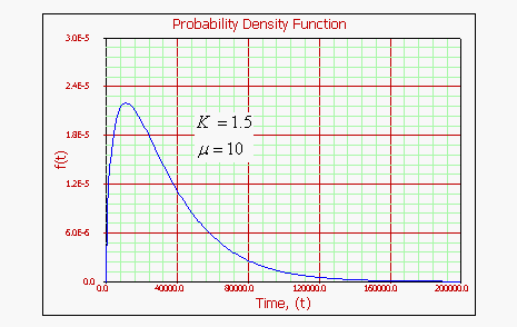
For $k>1$ :

• As $T\to 0,\mathrm{\infty }$ , $f(T)\to 0.$

• $f(T)$ increases from 0 to the mode value and decreases thereafter.

• If $k\le 2$ then $pdf$ has one inflection point at $T=e^{\mu }\sqrt{k-1}($ $\sqrt{k-1}+1).$

• If $k>2$ then $pdf$ has two inflection points for $T=e^{\mu }\sqrt{k-1}($ $\sqrt{k-1}\pm 1).$

• For a fixed $k$ , as $\mu$ increases, the $pdf$ starts to look more like a straight angle.

As $T\to \mathrm{\infty },\lambda (T)\to \frac{1}{e^{\mu }}.$

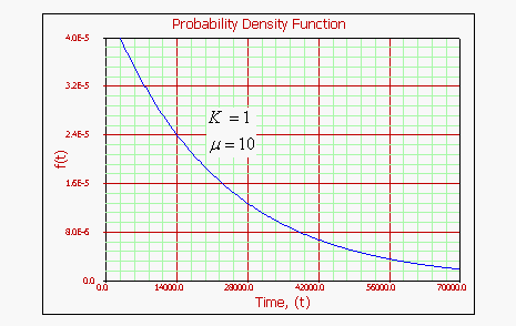
For $k=1$ :

• Gamma becomes the exponential distribution.

• As $T\to 0$ , $f(T)\to \frac{1}{e^{\mu }}.$

• As $T\to \mathrm{\infty },f(T)\to 0.$

• The $pdf$ decreases monotonically and is convex.

• $\lambda (T)\equiv \frac{1}{e^{\mu }}$ . $\lambda (T)$ is constant.

• The mode does not exist.

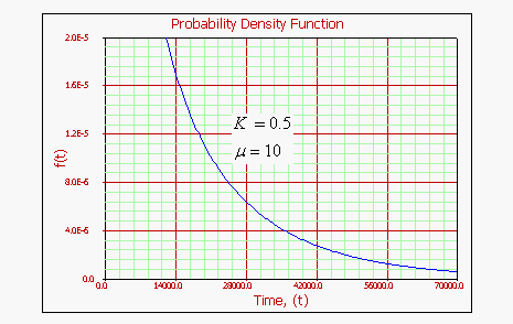
For $0<k<1$ :

• As $T\to 0$ , $f(T)\to \mathrm{\infty }.$

• As $T\to \mathrm{\infty },f(T)\to 0.$

• As $T\to \mathrm{\infty },\lambda (T)\to \frac{1}{e^{\mu }}.$

• The $pdf$ decreases monotonically and is convex.

• As $\mu$ increases, the $pdf$ gets stretched out to the right and its height decreases, while maintaining its shape.

• As $\mu$ decreases, the $pdf$ shifts towards the left and its height increases.

• The mode does not exist.

Confidence Bounds

The only method available in Weibull++ for confidence bounds for the gamma distribution is the Fisher matrix, which is described next. The complete derivations were presented in detail (for a general function) in Chapter 5.

Bounds on the Parameters

The lower and upper bounds on the mean, $\hat{\mu }$ , are estimated from:

$\begin{array}{rlr}& {\mu }_U=& \hat{\mu }+K_{\alpha }\sqrt{Var(\hat{\mu })}\text{ (upper bound)}\\ & {\mu }_L=& \hat{\mu }-K_{\alpha }\sqrt{Var(\hat{\mu })}\text{ (lower bound)}\end{array}$

Since the standard deviation, $\hat{\sigma }$ , must be positive, $\ln (\hat{\sigma })$ is treated as normally distributed and the bounds are estimated from:

$\begin{array}{rlr}& k_U=& \hat{k}\cdot e^{\frac{K_{\alpha }\sqrt{Var(\hat{k})}}{\hat{k}}}\text{ (upper bound)}\\ & k_L=& \frac{\hat{\sigma }}{e^{\frac{K_{\alpha }\sqrt{Var(\hat{k})}}{\hat{k}}}}\text{ (lower bound)}\end{array}$

where $K_{\alpha }$ is defined by:

$\alpha =\frac{1}{\sqrt{2\pi }}{\int }_{K_{\alpha }}^{\mathrm{\infty }}{e}^{-\frac{t^2}{2}}dt=1-\mathrm{\Phi }(K_{\alpha })$

If $\delta$ is the confidence level, then $\alpha =\frac{1-\delta }{2}$ for the two-sided bounds and $\alpha =1-\delta$ for the one-sided bounds.

The variances and covariances of $\hat{\mu }$ and $\hat{k}$ are estimated from the Fisher matrix, as follows:

$\left(\begin{array}{cc}\widehat{Var}\left(\hat{\mu }\right)& \widehat{Cov}(\hat{\mu },\hat{k})\\ \widehat{Cov}(\hat{\mu },\hat{k})& \widehat{Var}\left(\hat{k}\right)\end{array}\right)={\left(\begin{array}{cc}-\frac{{\partial }^2\mathrm{\Lambda }}{\partial {\mu }^2}& -\frac{{\partial }^2\mathrm{\Lambda }}{\partial \mu \partial k}\\ & \\ -\frac{{\partial }^2\mathrm{\Lambda }}{\partial \mu \partial k}& -\frac{{\partial }^2\mathrm{\Lambda }}{\partial k^2}\end{array}\right)}_{\mu =\hat{\mu },k=\hat{k}}^{-1}$

$\mathrm{\Lambda }$ is the log-likelihood function of the gamma distribution, described in Chapter 3 and Appendix C.

Bounds on Reliability

The reliability of the gamma distribution is:

$\hat{R}(T;\hat{\mu },\hat{k})=1-{\mathrm{\Gamma }}_1(\hat{k};e^{\hat{z}})$

where:

$\hat{z}=\ln (t)-\hat{\mu }$

The upper and lower bounds on reliability are:

$R_U=\frac{\hat{R}}{\hat{R}+(1-\hat{R})\exp (\frac{-K_{\alpha }\sqrt{Var(\hat{R})}}{\hat{R}(1-\hat{R})})}\text{ (upper bound)}$

$R_L=\frac{\hat{R}}{\hat{R}+(1-\hat{R})\exp (\frac{K_{\alpha }\sqrt{Var(\hat{R})}}{\hat{R}(1-\hat{R})})}\text{ (lower bound)}$

where:

$Var(\hat{R})={(\frac{\partial R}{\partial \mu })}^{2}Var(\hat{\mu })+2(\frac{\partial R}{\partial \mu })(\frac{\partial R}{\partial k})Cov(\hat{\mu },\hat{k})+{(\frac{\partial z}{\partial k})}^{2}Var(\hat{k})$

Bounds on Time

The bounds around time for a given gamma percentile (unreliability) are estimated by first solving the reliability equation with respect to time, as follows:

$\hat{T}(\hat{\mu },\hat{\sigma })=\hat{\mu }+\hat{\sigma }z$

where:

$z=\ln (-\ln (R))$

$Var(\hat{T})={(\frac{\partial T}{\partial \mu })}^{2}Var(\hat{\mu })+2(\frac{\partial T}{\partial \mu })(\frac{\partial T}{\partial \sigma })Cov(\hat{\mu },\hat{\sigma })+{(\frac{\partial T}{\partial \sigma })}^{2}Var(\hat{\sigma })$

or:

$Var(\hat{T})=Var(\hat{\mu })+2\hat{z}Cov(\hat{\mu },\hat{\sigma })+{\hat{z}}^{2}Var(\hat{\sigma })$

The upper and lower bounds are then found by:

$\begin{array}{rlr}& T_U=& \hat{T}+K_{\alpha }\sqrt{Var(\hat{T})}\text{ (Upper bound)}\\ & T_L=& \hat{T}-K_{\alpha }\sqrt{Var(\hat{T})}\text{ (Lower bound)}\end{array}$

A Gamma Distribution Example

Twenty four units were reliability tested and the following life test data were obtained:

$\begin{array}{cccccc}\text{61}& \text{50}& \text{67}& \text{49}& \text{53}& \text{62}\\ \text{53}& \text{61}& \text{43}& \text{65}& \text{53}& \text{56}\\ \text{62}& \text{56}& \text{58}& \text{55}& \text{58}& \text{48}\\ \text{66}& \text{44}& \text{48}& \text{58}& \text{43}& \text{40}\end{array}$

Fitting the gamma distribution to this data, using maximum likelihood as the analysis method, gives the following parameters:

$\begin{array}{rlr}& \hat{\mu }=& 7.72E-02\\ & \hat{k}=& 50.4908\end{array}$

Using rank regression on $X,$ the estimated parameters are:

$\begin{array}{rlr}& \hat{\mu }=& 0.2915\\ & \hat{k}=& 41.1726\end{array}$

Using rank regression on $Y,$ the estimated parameters are:

$\begin{array}{rlr}& \hat{\mu }=& 0.2915\\ & \hat{k}=& 41.1726\end{array}$